Conway’s Game of Life is a simple simulation with surprisingly complex behavior. We start with a simple 2D grid of cells. Each cell can be either alive or dead. The rules are:
We started with a certain set of cell states and then iterate, applying the rules to every cell at each iteration. Despite their simplicity, these rules can produce amazingly complicated behavior. For example, here is Gosper’s Glider Gun, which produces “gliders” which wander off to infinity:1
For our Statistical Computing course, Chris Genovese used the Game of Life as an example at the very beginning of the course to illustrate the flexible design of programs. Students first were told to write an ordinary implementation following the rules above – then asked how they’d abstract their algorithm so they could replace the rules or even work on a non-rectangular grid. Without careful planning, that kind of abstraction could be very difficult.
So here’s a sample implementation in Racket, my favorite little Lisp.
First we need to specify the rules of the game. Conway’s rules are the most popular, but it’s possible to use different rules to decide which cells live or die, so we’ll abstract the rules out to a function.
The rules function only needs to know two things: the number of neighbors the cell has, and whether or not it’s currently alive. Then it returns a boolean indicating whether the cell will stay alive.2
(define (conway-rules neighbors alive?)
  (if alive? (or (= neighbors 2) (= neighbors 3))
      (= neighbors 3)))
If we want to try out different sets of rules, it’s easy to define entirely new functions – with arbitrary logic and complexity – which can replace conway-rules. As you’ll see below, conway-rules is passed as an argument to our other functions, so replacing it requires no source code changes at all.
It’s tempting to store the state of the Game of Life using some kind of two-dimensional array or matrix. Then, on each step, we’d loop through the whole board, checking which cells should live or die. But this would become slow – the gliders we saw earlier can wander off arbitrarily far, so our board would have to be large and the loop slow. If our board isn’t large enough, cells could reach the edge, and we’d either need to increase the board size or accept that their behavior will be wrong.
Worse, the amount of computation needed would grow with the board size, regardless of how many cells in the board are actually alive. In the worst case, we’d have an enormous board of entirely dead cells, and at every step we’d still loop through the whole thing checking if anything should come alive.
But look back at the rules. All we really need to keep track of is the live cells. We can tell if a cell comes alive just by knowing if it has live neighbors.
Imagine we have a list of currently live cells. If we find the neighbors of each live cell, we’ll have a big list of coordinates; if a cell is the neighbor of three live cells, it’ll appear in that list three times. So, for example, a currently dead cell which is the neighbor of three live cells will appear in the list, and we can mark it as alive on the next step.
On our rectangular grid, we can easily find the neighbors of a single cell with
(define (neighbors-rect location)
  (let ([x (first location)]
        [y (last location)])
    (for*/list ([dx '(-1 0 1)]
                [dy '(-1 0 1)]
                #:when (not (= dx dy 0)))
      (list (+ x dx) (+ y dy)))))
Coordinates are stored as (x, y) pairs. We loop through perturbations, adding or subtracting 1 from x and y, generating the eight neighbor coordinates.
I’m going to put together a key function from a few pieces here. Let’s start with the basic bits. To apply Conway’s rules, we start by getting the list of all neighbors of all cells:
We need to count how many times each coordinate appears in this list, so we’ll use a hash table. The result is a table of item,count pairs:
(define (count-occurrences neighbors)
  (for/fold ([ht (hash)])
            ([item neighbors])
    (hash-update ht item add1 0)))
hash-update takes a hash table, looks for a key (item), and updates it according to the function passed to it – in this case add1, so the count is incremented by 1. If the key doesn’t exist, we pass 0 to add1 as the default. As a result, we have a count of how many time each item appears in the neighbors list.
Then it’s just a matter of applying the rules. If we have the number of neighbors and a set of live cells, then applying the rules is as simple as
The hash-ref simply looks up the cell in the table, returning how many neighbors it has.
Now we can assemble together a function to take a set of live cells and return a new set:
Our step function only runs one iteration: it applies the rules, generates the new set of live cells, and returns it. How do we run the Game of Life for more steps?
A simple route would be a for loop. But we can be fancier. Racket supports lazy sequences: infinitely long sequences whose elements are calculated only when we ask for them. We can define one recursively.
stream-cons is an interesting function that works recursively. It defines a stream (a sequence) that begins with cells and whose next element is formed by calling its second argument – which creates another sequence that starts at the next step.
In summary, life applies Conway’s rules on a rectangular grid, making an infinite sequence of cell states. We can ask Racket to provide any element in the sequence and it’ll be calculated on demand.
Let’s try our code on a sample set of live cells. We’ll use the “acorn”, a configuration which starts small and then grows for thousands of generations. I’ve imported a draw-game function which draws the results. At the beginning, it looks like this:

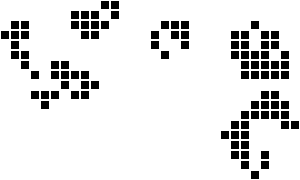
But after just fifty steps, we have:
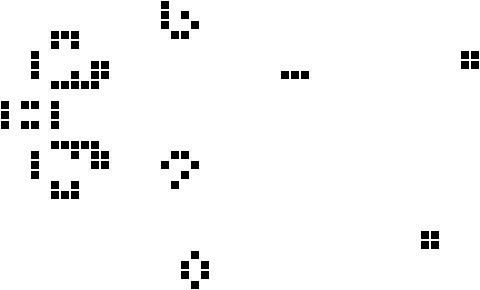
And after fifty more:
One more thing. Previously we defined a neighbors function, which gets the list of neighbors of a cell. That function assumed we were working on a rectangular grid. But, if you look carefully, you’ll see it’s the only function which assumes that. If we want to change the grid, we need only swap out the neighbors function.
Suppose, then, we swap out the rectangular grid for a hexagonal one. There are many possible hexagonal grid coordinate systems, so I’ve chosen one arbitrarily, and to make it brief, each cell has six neighbors instead of eight, and we can generate them all with a slightly different function:
(define (neighbors-hex location)
  (let ([x (first location)]
        [y (last location)])
    (for*/list ([dx '(-1 0 1)]
                [dy '(-1 0 1)]
                #:when (and (not (= dx dy 1))
                            (not (= dx dy -1))
                            (not (= dx dy 0))))
      (list (+ x dx) (+ y dy)))))
By swapping out neighbors-rect for neighbors-hex in our definition of life, we can work on a hexagonal grid. No other code needs to change except for how we draw the grid.
Animation from Wikimedia Commons.↩
I apologize for the minimal syntax highlighting. pandoc’s syntax highlighting library doesn’t support Racket yet, so I’m using the Clojure highlighting, which doesn’t recognize most of Racket’s keywords.↩