13 Observational Design

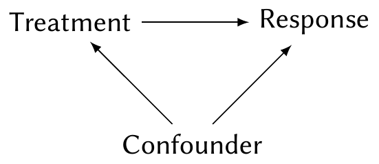
In Chapter 2, we discussed the standard reason to do an experiment. Suppose we want to know the effect of a treatment on a response, but there is a confounder:

By randomly assigning treatment, we can break the arrow from the confounding variable to treatment, thus allowing us to estimate the effect of treatment on response. To get the best possible estimate, we used all our experimental design techniques, such as blocking and control of covariates.

What if we can’t assign the treatment? We then have an observational study, so we are limited to measuring associations—but if we are willing to make some assumptions, and if we observe the relevant confounding variables, we may be able to get close to the causal effect.

Consider the case where the treatment is binary, so we can denote it as \(Z_i \in \{0, 1\}\). Let \(\pi_i = \Pr(Z_i = 1 \mid X_i = x_i)\) for each unit \(i\), where \(X_i\) are the covariates (including the confounders). In an experiment, \(\pi_i\) is under our control: we choose it based on our design, and it reflects the randomization procedure we select. Because we choose it, there is no arrow from confounder to treatment.

But in an observational study, \(\pi_i\) may depend on the confounder. It may be unknown: we do not know how the confounder affects the treatment, just that it does. How it varies matters. If \(\pi_i = 0.5\) for all \(i\), then the confounder has no effect on the treatment, and it is not a confounder at all—so we may safely conclude association is causation. If \(\pi_i\) is larger for people who will respond well to the treatment and smaller for people who won’t, then on average, the people who receive the treatment will also have a better response, and we will overestimate its effect.

Suppose, then, that we could estimate \(\pi_i\) and extract out everyone with a similar value of it. We could then take a subgroup for whom, say, \(\pi_i \approx 0.4\). Within this group, the confounder does not affect the treatment, and so we may estimate the association between treatment and response. We could repeat this for subgroups with \(\pi_i \approx 0.5\), \(\pi_i \approx 0.6\), and so on, and combine the results to form an estimate of the overall effect.

That suggests several possible strategies to estimate a causal effect, even in an observational study:

Attempt to model \(\pi_i\) and then group together units with similar values. Conduct analysis within each group. This is a stratified analysis.
Match up units with \(Z_i = 0\) and \(Z_i = 1\) that have similar values of \(\pi_i\). Compare each treated unit to its companion control unit. This is called matching.
Build a model to estimate \(\pi_i\) and use the predicted values in your model as a control variable.

Each of these has its uses. Let’s start with the foundations.

13.1 Propensity scores

Let’s redefine \(\pi_i\) as a propensity score. In general, the probability of treatment may depend on both observed covariates and unobserved covariates, and perhaps even the potential outcomes \(C_i(Z_i)\), so let’s include all of those.

Definition 13.1 (Propensity score) In an observational study with treatment binary \(Z_i\), observed covariates \(X_i\), unobserved covariates \(U_i\), and potential outcomes \(C_i\), the propensity scores are the values \[ \pi_i = \Pr(Z_i = 1 \mid X_i = x_i, U_i = u_i, C_i(0), C_i(1)). \] We interpret them as the propensity to receive the treatment (\(Z_i = 1\)) given all the factors that may influence it.

We can think of the propensity scores as summarizing all the information (contained in the covariates) relevant to whether or not you receive the treatment. TODO show concretely that these are sufficient to estimate the causal effect from the observed data

Suppose the observed covariates \(X_i\) are the only things that affect the probability of treatment—there are no unobserved confounders and there is no relationship between treatment and the counterfactuals. In this situation, we say the treatment assignment is “strongly ignorable” given \(X\).

Definition 13.2 (Strong ignorability) If the propensity score (Definition 13.1) can be written as \[ \pi_i = \Pr(Z_i = 1 \mid X_i = x_i), \] without unobserved confounders or potential outcomes, if \(0 < \pi_i < 1\) for all \(i\), and if the treatment assignments are conditionally independent given \(X\), we say the treatment assignment is strongly ignorable given the observed covariates \(X\).

Example 13.1 (Strongly ignorable experiments)

In a Bernoulli experiment (Definition 4.3), \(\pi_i = p\) for all \(i\), so treatment assignment is strongly ignorable (and doesn’t even depend on \(X\)).
In an experiment blocked on the covariates \(X\), the treatment assignment depends on \(X\) but nothing else, and is strongly ignorable.

As we will see below, if the treatment assignments are strongly ignorable, we can simply perform matching: match up two units with \(Z_i = 0\) and \(Z_i = 1\) whose values of \(X\) are nearly identical. Their difference in response should estimate the causal effect. This is exactly how estimation is done in, say, a blocked experiment, where we compare treatments within levels of our blocks.

We can’t test strong ignorability from the observed data, as we can’t test the association between \(Z_i\) and unobserved data without observing it. Judging whether it holds depends on your understanding of the assignment mechanism. (Which is why designed experiments are so useful!)

Regardless of whether the strong ignorability assumption holds, the propensity score based on the observed covariates summarizes all the information about them that is relevant to assignment.

Theorem 13.1 (Balancing property) The treatment and covariates are conditionally independent given the propensity score: \[ Z_i \perp X_i \mid \lambda(x_i), \] where \(\lambda(x)\) is the propensity score function on the observed covariates: \[ \lambda(x) = \Pr(Z = 1 \mid X = x). \]

Proof. The independence means that \[ \Pr(X = x \mid \lambda(x) = \lambda, Z = 1) = \Pr(X = x \mid \lambda(x) = \lambda, Z = 0). \] We can show this is true with Bayes’ theorem: \[\begin{align*} \Pr(X = x \mid \lambda(x) = \lambda, Z = 0) &= \frac{\Pr(Z = 1 \mid \lambda(x) = \lambda, X = x) \Pr(X = x \mid \lambda(x) = \lambda)}{\Pr(Z = 1 \mid \lambda(x) = \lambda)}\\ &= \frac{\lambda \Pr(X = x \mid \lambda(x) = \lambda)}{\lambda}\\ &= \Pr(X = x \mid \lambda(x) = \lambda). \end{align*}\] So the distribution of \(X\) is independent of \(Z\), conditional on \(\lambda(x)\).

The propensity score function \(\lambda(x)\) is in principle unknown, but it can be estimated from the observed data. If we observe \(X\) and \(Z\), we need only fit a binary classifier, such as logistic regression, to obtain \(\hat \lambda(x)\).

13.2 Matching

To estimate the causal effect despite confounders, our first intuition may be to condition on (control for) the confounders. That could be with a model, but a simpler approach is to group units with similar values. Just as in blocking, we can take all units with a particular value of \(X\) and compare the treated and untreated ones, then repeat for different values of \(X\). However, this becomes difficult when we have many covariates, just as blocking gets complicated when we have many blocking variables, and it can be difficult to exactly match a treated unit with particular \(X\) to an exactly comparable untreated unit.

According to the balancing property, conditioning on \(\lambda(x)\) makes \(Z\) and \(X\) independent. Thus it is sufficient to match on propensity scores instead, and propensity scores are univariate—no fancy multivariate matching required. However:

We only have \(\hat \lambda(x)\), not \(\lambda(x)\).
It may not be possible to exactly match on \(\lambda(x)\), or only possible for a subset of units. When \(\lambda(x) > 0.5\), we’ll have more treatment units than control units, and when \(\lambda(x) < 0.5\) we’ll have the reverse; thus there may not be enough treatment and control units to exactly match at each level.
If there are units where \(\lambda(x) = 0\) or \(\lambda(x) = 1\), there will be no units with the opposite treatment! Every unit with \(\lambda(x) = 1\) got treated, so there are no controls they can be matched to.

Propensity score matching strategies hence cannot and do not match on \(\lambda(x)\) (or \(\hat \lambda(x)\)) exactly. There are many strategies. A common one is to match the propensity scores using a caliper, which means choosing a width \(w\) and only matching units where \(|\hat \lambda(x_i) - \hat \lambda(x_j)| < w\). Among pairs of units whose estimated propensity scores are within this caliper width, we use a measure of distance between their \(x\) values, such as the Mahalanobis distance, to pair the closest treatments and controls.

There are also optimization-based approaches, known as optimal pair matching, that treat this as a combinatorial optimization problem to find the pairing that minimizes the total distances between treatment and control in each pair.

13.3 Inverse propensity score weighting

Besides matching, we can use the propensity scores in another way.

Theorem 13.2 (Inverse propensity weighting) In a strongly ignorable binary experiment with treatment \(Z_i\), counterfactuals \((C_i(0), C_i(1))\), and response \(Y_i\), the average treatment effect (Definition 6.1) can be written as \[ \E[C_i(1) - C_i(0)] = \E\left[ \frac{Z_i Y_i}{\lambda(X_i)} - \frac{(1 - Z_i) Y_i}{1 - \lambda(X_i)}\right], \] where \(X_i\) are the observed covariates and \(\lambda(X_i)\) is the propensity score.

Proof. Using linearity of expectations, we can split the right-hand side in two. Consider each part. First, by the law of total expectation, \[\begin{align*} \E\left[ \frac{Z_i Y_i}{\lambda(X_i)} \right] &= \Pr(Z_i = 1) \E\left[ \frac{1 Y_i}{\lambda(X_i)} \mid Z_i = 1 \right] + \Pr(Z_i = 0) \E\left[ \frac{0 Y_i}{\lambda(X_i)} \mid Z_i = 0 \right] \\ &= \frac{\Pr(Z_i = 1)}{\lambda(X_i)} \E[C_i(1)]\\ &= \E[C_i(1)], \end{align*}\] by definition of the propensity score under strong ignorability.

For the second term, we can do a very similar trick and get \(\E[C_i(0)]\), proving the desired result.

This leads to a simple estimator.

Definition 13.3 (Horvitz–Thompson estimator) The Horvitz–Thompson estimator of the average treatment effect is \[ \hat \tau_{\text{IPW}} = \frac{1}{n} \sum_{i=1}^n \left( \frac{Z_i Y_i}{\hat \lambda(X_i)} - \frac{(1 - Z_i) Y_i}{1 - \hat \lambda(X_i)} \right). \]

If we have a good estimate of the propensity scores, this is easy to do. It is less fiddly than matching, which can involve complicated optimization problems and may leave us with some units we cannot match; it is also unbiased when the assumptions hold. However, anything involving ratios where an estimator is in the denominator should make you nervous: if \(\hat \lambda(X_i) \approx 0\) or \(\hat \lambda(X_i) \approx 1\) for one or more units, some of these denominators can be arbitrarily small, “blowing up” that term in the sum.

On the one hand, this makes sense: If \(\lambda(X_i) \approx 1\), it is almost impossible for us to observe \(C_i(0)\), so we will have very little data to estimate \(C_i(1) - C_i(0)\). But it is very inconvenient. Because \(\hat \lambda\) is only an estimate, we expect it to have some uncertainty, and we can end up with extreme values. Those terms make \(\var(\hat \tau_{\text{IPW}}\) very big.

13.4 Outcome regression

TODO Just do \(\E[Y \mid X, Z]\)

13.5 Doubly robust estimation

TODO