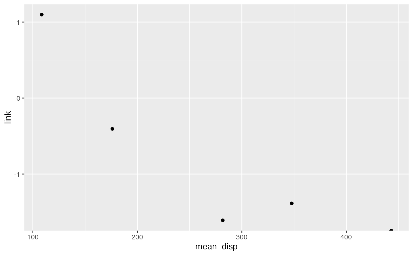
Empirically estimate response values on the link scale — empirical

Calculates the average value of the response variable, and places this on the link scale. Plotting these against a predictor (by dividing the dataset into bins) can help assess the choice of link function.

Usage

empirical_link(response, family, na.rm = FALSE)

Arguments

response: Vector of response variable values.
family: Family object representing the response distribution and link function. Only the link function will be used.
na.rm: Should NA values of the response be stripped? Passed to mean() when calculating the mean of the response.

Value

Mean response value, on the link scale: $g(\bar Y)$, where $\bar Y$ is the mean of response.

Details

A generalized linear model is one where $Y$ is modeled with some parametric distribution (such as binomial or Poisson) conditional on $X$, and

$$g(\mathbb{E}[Y \mid X = x]) = \mu(x)$$

where $g$ is a link function.

In exploratory data analysis, we can plot $X$ against $g(Y)$ to evaluate whether the model is adequate. Typically this is done by binning the data (for example, by values of $X$), taking the average of $Y$ in each bin, and then using $g$ to transform the average.

This can be used to make empirical link plots; see vignette("other-glm-diagnostics").

Examples

suppressMessages(library(dplyr))
suppressMessages(library(ggplot2))

# An empirical link plot for `am`, assuming a binomial with logit link:
mtcars |>
  bin_by_interval(disp, breaks = 5) |>
  summarize(
    mean_disp = mean(disp),
    link = empirical_link(am, binomial())
  ) |>
  ggplot(aes(x = mean_disp, y = link)) +
  geom_point()