The regressinator is a pedagogical tool for conducting simulations of regression analyses and diagnostics. It can:
- Simulate populations with predictor variables from arbitrary distributions
- Simulate response variables that are functions of the predictor variables plus error, or are drawn from a distribution related to the predictors
- Given a model, simulate from the population sampling distribution of that model’s estimates
- Given a model fit to data, generate new simulated data based on the model fit
- Facilitate lineup plots comparing diagnostics on the fitted model to diagnostics where all model assumptions are met.
These features make it easy to create activities and examples for classes teaching regression using R. Lineup plots are great for helping students understand how regression diagnostics behave with different types of model misspecification, and for more advanced classes, simulating from sampling distributions helps students explore the properties of regression estimators. And the easy simulation features aren’t just useful for students—instructors can easily generate examples for lectures, exams, and labs.
For example, suppose we want to teach students how residual plots look when a linear regression is fit to nonlinear data. We can quickly specify a nonlinear relationship and generate a lineup plot that hides the residual plot among 19 others where the model assumptions are met:
library(regressinator)
library(ggplot2)

# define the population relationship
pop <- population(
  x = predictor(runif, min = -5, max = 5),
  y = response(10 + 0.7 * x**2, family = gaussian(), error_scale = 2)
)

# obtain a random sample from the population
nonlin_sample <- pop |>
  sample_x(n = 20) |>
  sample_y()

# fit a model to the sample
fit <- lm(y ~ x, data = nonlin_sample)

# construct a lineup, with 19 models fit to data simulated from the linear model
model_lineup(fit) |>
  ggplot(aes(x = x, y = .resid)) +
  geom_point() +
  facet_wrap(vars(.sample)) +
  labs(x = "x", y = "Residual")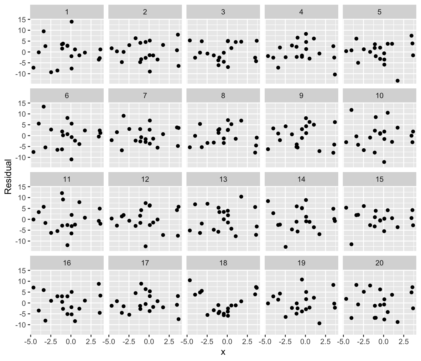
If you can identify the “true” residual plot from the lineup, you have found model misspecification. This lineup is essentially a visual hypothesis test, and it helps students see the variation expected in diagnostics and what nonlinear trends look like. (For more on lineups and how they can be used in teaching, see Inspirations below.) model_lineup() achieves this by simulating 19 datasets from the fitted model (so the relationship is truly linear), then broom::augment() to obtain the data and residuals from each fit.
Similarly, we can quickly obtain samples from the population sampling distribution, to explore the behavior of this misspecified model’s parameter estimates:
fit |>
  sampling_distribution(nonlin_sample, nsim = 5)
## # A tibble: 12 × 6
## term estimate std.error statistic p.value .sample
## <chr> <dbl> <dbl> <dbl> <dbl> <dbl>
## 1 (Intercept) 15.7 0.991 15.9 4.98e-12 0
## 2 x 0.164 0.330 0.496 6.26e- 1 0
## 3 (Intercept) 16.4 1.01 16.3 3.24e-12 1
## 4 x 0.0746 0.335 0.223 8.26e- 1 1
## 5 (Intercept) 16.7 1.22 13.7 5.71e-11 2
## 6 x 0.0977 0.405 0.241 8.12e- 1 2
## 7 (Intercept) 17.3 1.30 13.3 9.86e-11 3
## 8 x 0.0796 0.433 0.184 8.56e- 1 3
## 9 (Intercept) 15.4 0.956 16.1 3.92e-12 4
## 10 x -0.0483 0.318 -0.152 8.81e- 1 4
## 11 (Intercept) 15.6 1.18 13.3 9.70e-11 5
## 12 x -0.0155 0.391 -0.0397 9.69e- 1 5Here sampling_distribution() defaults to using broom::tidy() to obtain the coefficients and standard errors for each fit. We could use this to assess bias, to compare the sampling distribution to standard errors and confidence intervals, or simply to visualize variation.
The premise of the regressinator is that this kind of simulation can be a valuable teaching tool when students are learning to interpret regression diagnostics and determine how different kinds of misspecification might affect model fits.
Check the Get Started guide (vignette("regressinator")) for more detail.
Inspirations
Visual inference – hiding a plot of real data among “null plots” – has been around for quite a while, and I certainly did not invent this idea myself. For example:
Buja, A., Cook, D., Hofmann, H., Lawrence, M., Lee, E. K., Swayne, D. F., & Wickham, H. (2009). Statistical inference for exploratory data analysis and model diagnostics. Philosophical Transactions of the Royal Society A, 367(1906), 4361–4383.
Wickham, H., Cook, D., Hofmann, H., & Buja, A. (2010). Graphical inference for infovis. IEEE Transactions on Visualization and Computer Graphics, 16(6), 973–979.
Loy, A., Follett, L., & Hofmann, H. (2016). Variations of Q-Q Plots: The Power of Our Eyes! The American Statistician, 70(2), 202–214.
The idea of using visual inference to teach regression diagnostics is also not new:
- Loy, A. (2021). Bringing Visual Inference to the Classroom. Journal of Statistics and Data Science Education, 29(2), 171-182.
The regressinator simply adds an easy-to-use framework to allow all kinds of teaching activities to be constructed quickly. Instructors can design example to display in lecture, or students with R experience can run interactive examples and explore different situations. Ideally, if a student asks “But what if [some problem with the model] happens?”, you should be able to reply with a quick simulation.
Compared to other packages
There have been several past efforts to support pedagogical simulation and lineup plots in R:
- nullabor, which supports lineup plots. The regressinator uses nullabor underneath when building lineups.
-
mosaic, part of Project MOSAIC, provides a simple set of functions for doing EDA and basic inferential statistics, including the
do()function for easy simulation without loops. - infer, part of the tidymodels framework, can conduct simulation-based inference for proportions, means, regression slopes, and other estimates commonly used in statistics courses, using only a few simple functions.
Unlike these packages, the regressinator provides a simple tool for specifying a population and sampling from it, rather than conducting bootstrapping or permutation on an observed dataset. This makes the regressinator suitable for, say, exploring the properties of regression estimates and diagnostics in known populations, but less suitable for simulation-based hypothesis testing.
Unlike infer, the regressinator does not wrap R statistical methods or provide its own inference functions. Users must use lm(), glm(), or whatever other methods they need for their modeling. This makes the regressinator less suitable for introductory courses where extra complexity should be hidden away from students, but more suitable for more advanced work: as students advance to more complex models provided by other packages, they can use those models in the regressinator, without any special support being required.
A useful counterpart to the regressinator might be rsample, a general framework for methods that resample from the observed data, such as bootstrapping. In the same way that the regressinator supports general-purpose simulation from the population without hard-coding specific use cases, rsample supports resampling and cross-validation in a general way that could be used for any kind of modeling, not just models built into the package.