19 Introduction to Neural Networks
\[ \DeclareMathOperator{\E}{\mathbb{E}} \DeclareMathOperator{\R}{\mathbb{R}} \DeclareMathOperator{\softmax}{softmax} \DeclareMathOperator*{\argmin}{argmin} \newcommand{\T}{^\mathsf{T}} \]
Deep learning is currently the hottest topic in machine learning. The fundamental ideas come from at least the 1950s, and neural networks were briefly popular in the 1990s, but it’s only since about 2010 that events have come together to make deep learning popular: a massive flood of training data (i.e. the Internet) and powerful computers that can handle it.
What is deep learning? Broadly, we can think of it as a very flexible way to build regression and classification models.
Note
Portions of this page are based on materials from Max G’Sell and Christopher Genovese, whose courses I have taught or co-taught.
19.1 Flexible regression
Consider simple linear regression. We observe features \(X \in \R^p\) and outcomes \(Y \in \R\). We choose a linear regression model that says \[ Y = X \beta + \epsilon, \] and we estimate \(\beta\) by solving the least squares problem: \[ \hat \beta = \argmin_\beta \sum_{i=1}^n (Y_i - X_i\T \beta)^2. \] That works well when the true regression function is approximately linear. If it’s not, we have various approaches: transformations, splines, regression trees, kernel regression, and so on.
Transformations like logs and polynomials are a good example of feature engineering: improve your results by trying to improve your feature vector \(X\). If we make a function \(\phi(x) = (\phi_1(x), \dots, \phi_K(x))\) that calculates \(K\) custom features, we can fit the model \[ Y = \phi(X) \beta + \epsilon \] using the same least squares procedure.
You’ve done this before. And in many applications, graduate students spent years of labor choosing \(\phi\). In image recognition, where \(X\) is an image, there was much work on functions \(\phi\) that could take an image as input and extract features: edge detectors, corner detectors, keypoint finders, and so on. In speech recognition, where \(X\) is an audio recording, there was much work on spectrograms and signal processing to extract and classify syllables.
But if we could estimate \(\phi(X)\) from the data, we could replace feature engineering. We could let \(\phi(X; \theta)\) be a function of additional parameters \(\theta \in \R^d\), and estimate those too.
Exercise 19.1 (Why not linear?) What if we chose \(\phi(X; \theta) = \theta X\), where \(\theta\) is a \(q \times p\) matrix of new parameters? Then we generate a vector of new covariates.
Can this improve our regression model?
Instead of linear functions, a common choice is to let \[ \phi_j(X, \theta_j) = g(X\T \theta_j + c_j). \] Here \(g\) is a nonlinear activation function, \(\theta_j\) is a vector of weights, and \(c_j\) is a scalar bias. We use functions \(\phi_1, \dots, \phi_K\), and hence have a weight matrix \(\theta \in \R^{K \times p}\) and a bias vector \(c \in \R^K\).
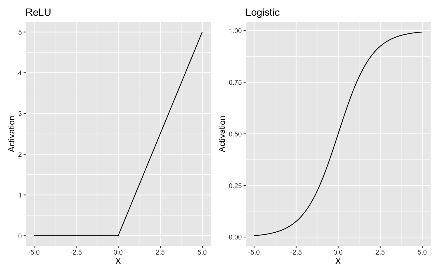
Two common activation functions (we’ll see more in Section 19.3.2) are the rectified linear unit (ReLU) and the logistic: \[\begin{align*} g(x) &= \max\{0, x\} & \text{ReLU}\\ g(x) &= \frac{1}{1 + e^{-x}} & \text{logistic}. \end{align*}\]
If we use these to produce new features, we end up with a model of the form \[ Y = \sum_{i=1}^K \beta_k g(X\T \theta_k + c_k) + \epsilon. \] Surprisingly enough, the universal approximation theorem says that if we set \(K\) large enough, and use an activation function such as the logistic, this approach can approximate any Borel measurable function to any desired degree of error (Hornik, Stinchcombe, and White 1989; Cybenko 1989). Provided, of course, that we can find good values of \(\theta\) and \(c\).
19.2 The neural metaphor
The model above is actually a very simple example of a feed-forward neural network. Neural networks were inspired by analogies to real brains, although they are more like a simplified analogy of a small fraction of brain function than artificial brains. Nonetheless, the idea of “neurons” and their interconnection gives us a simple way to visualize what this model is doing.
[TODO neural diagram]
Example 19.1 (A simple feed-forward network) TODO diagram of the model presented above, labeled
This suggests we can build a network recursively, by adding successively more hidden layers.
Why add more layers when the universal approximation theorem says we only need one really big layer? The theorem says we can approximate any function to a desired degree of error, but it does not say it will be easy to find the weights and biases that produce the approximation function. The necessary hidden layer may also be ridiculously large, requiring so many parameters that the model is very easy to overfit.
Multiple smaller layers can often achieve the same flexibility with a computationally simpler and easier-to-fit network; and as we will see in TODO, using different types of layers will allow us to encode information about the problem into the model, giving it a head start on finding a solution.
See Goodfellow, Bengio, and Courville (2016), section 6.4.1, for a more detailed discussion of the research literature on layer counts, layer sizes, and performance.
We can also think of using multiple smaller layers as encoding a statistical belief about the problem to be solved. If we have multiple hidden layers, but one of those hidden layers has only 3 nodes, then our network transforms the data (through nonlinear activation functions) down to a vector of 3 numbers. If this works well, it implies the \(p\)-dimensional input data can be represented as a 3-dimensional summary that still provides adequate performance. In conventional regression, we often impose structure through sparsity, saying that most variables have no effect and only a few matter; in a neural network with a small internal hidden layer, all variables may matter, but only through a few particular nonlinear transformations of those variables.
19.3 Multi-layer feed-forward neural networks
A multi-layer feed-forward neural network has multiple hidden layers. It is feed-forward because all the values proceed from one layer to the next; later, we will see networks that are recurrent, meaning some values actually move backwards through the network.
19.3.1 Layer types
We can think of there being several types of layers in a neural network. Broadly, there are three categories:
- Input layer. The input layer has \(p\) nodes, where the covariates are \(X \in \R^p\). Each node represents one entry in the feature vector.
- Hidden layers. The hidden layers are the internal layers that do transformations of the input. These are typically nonlinear, and there are many specific types of input layers.
- Output layer. The output layer transforms the final hidden layer into the desired output: a single scalar value for regression, or
For example, in Example 19.1, the input layer has \(p\) nodes, the hidden layer has \(K\) nodes, and the output layer has 1 node.
The simplest type of layer is a fully connected layer. In a fully connected layer, all nodes have connections to all nodes in the previous layer. The layers in Example 19.1 are fully connected
19.3.2 Activation functions
\[\begin{align*} g(x) &= x & \text{identity/linear} \\ g(x) &= \max\{0, x\} & \text{ReLU}\\ g(x) &= \frac{1}{1 + e^{-x}} & \text{logistic/sigmoid} \\ g(x) &= \tanh(x) = \frac{\exp(x) - \exp(-x)}{\exp(x) + \exp(-x)} & \text{hyperbolic tangent} \end{align*}\]
The logistic link, also known as the sigmoid link, used to be very popular. However, when \(x\) is very large or very small, the link is nearly flat; that means the gradient of the loss with respect to the parameters (weights and biases) may be very small. Only a very small part of the logistic link’s range has larger derivatives, making it easy for gradient descent to get “stuck” making very slow progress.
The ReLU activation is most commonly used now, and is a good default starting point.
In Example 19.1, we could choose any nonlinear activation function for the hidden layer, while the output layer is a linear layer.
Activation functions are often written as vectorized functions, much like functions in R: \(g(x)\) when \(x \in R^p\) is interpreted as the mapping \(g(x) : \R^p \to \R^p\), applying the activation function separately to each entry in \(x\). This leads to some useful notation.
19.3.3 Simple notation for networks
We can often write neural networks in a simpler mathematical form. Let \(x \in \R^p\) be the contents of the input layer. The first hidden layer’s values are \[ h^{(1)} = g^{(1)} \left( (W^{(1)})\T x + b^{(1)} \right), \] where \(g^{(1)}\) is its activation function, \(W^{(1)} \in \R^{p \times l^{(1)}}\), \(b^{(1)} \in \R^{l^{(1)}}\), and \(l^{(1)}\) is the size of the first hidden layer. In this form, the weights for each node become a weight matrix, and the biases combine into a vector. Subsequent hidden layers are calculated by \[ h^{(k)} = g^{(k)} \left( (W^{(k)})\T h^{(k - 1)} + b^{(k)} \right), \] all the way to the output layer.
19.3.4 Output layers
Output layers can, in principle, be of any of the same types as hidden layers. Generally we choose the output layer to produce whatever output will be used in our loss function. In a regression problem, then, the output layer is typically a single node, representing the predicted scalar value.
In a binary classification problem, we might instead choose a logistic output layer with a single node, because the logistic output unit maps its input to the range \((0, 1)\). We can then treat the output as a predicted probability.
In a multiclass classification problem, we could use the softmax output layer. Suppose there are \(C\) classes. We create \(C\) output nodes, fully connected to the previous layer, and using the set of activation functions \[ \softmax(x)_i = \frac{\exp(x_i)}{\sum_{j=1}^C \exp(x_j)}. \] By definition, \[ \sum_{i=1}^C \softmax(x)_i = 1, \] and each entry is in the interval \((0, 1)\).
19.3.5 Loss functions
When fitting a model, we use some kind of objective function or criterion to determine what makes a good fit, then optimize that function to get our fit. You’ve done this many times before: the likelihood is an objective function, and maximizing it yields the maximum likelihood estimator.
Typically, we want to minimize some kind of loss when our function is applied to the population. That is, if our function is \(f(x; \theta)\), and \((x, y)\) come jointly from some distribution \(P\), we want to find \[ \hat \theta = \argmin_\theta \E_{(x, y) \sim P} L(f(x; \theta), y), \] where \(L(\hat y, y)\) is a loss function. For example, in linear models, we often use \[ L(\hat y, y) = (\hat y - y)^2, \] and so we want to find \(\hat \beta\) that minimizes the mean squared error: \[ \hat \beta = \argmin_\beta \E_{(x,y) \sim P} (X \beta - Y)^2. \] In a logistic regression where \(y \in \{0, 1\}\), we might instead use the loss \[ L(\hat y, y) = - y_i \log(\hat y_i) - (1 - y_i) \log(1 - \hat y_i), \] which is the (negative) Bernoulli log-likelihood function.
For multiclass classification problems, we can make a multinomial version of the loss; and, in general, we can be creative about loss functions when training neural networks to solve different problems.
These loss functions are applied to the output layer of the neural network during training and used during training. Let’s discuss training next.
19.4 How to train your model
Fitting a neural network, i.e. finding the parameters \(\theta\) that result in \(f(x; \theta)\) being a good approximator, is usually called training. The quantity we are minimizing—the expected loss on samples drawn from the population—is known as the risk. But of course we do not know the population distribution \(P\). We can instead minimize the empirical risk, which is the risk on our training sample: \[ \hat \theta = \argmin_\theta \frac{1}{n} \sum_{i=1}^n L(f(x_i; \theta), y_i). \] This is known as empirical risk minimization. The assumption is that our training sample is a representative sample from \(P\), so this minimizer will be an approximation of the risk minimizer.
For example, if our loss function were a negative log-likelihood function, empirical risk minimization would mean minimizing the negative log-likelihood on the training data—-or maximizing the likelihood on the training data.
In neural networks, we use gradient descent to implement this minimization efficiently. Unlike many kinds of mathematical optimization, however, we’re not always interested in reaching a true global—or even local!—minimum. Minima often overfit and produce models that fit very well to the training data and poorly to anything else, and so there are a variety of strategies to optimize without optimizing too much. We’ll discuss these later.
19.4.1 Batch and stochastic gradient descent
When we train a neural network with gradient descent, calculating the gradient requires calculating the gradient of each term in the sum. That is doable—back-propagation can handle sums as easily as anything else—but requires computation proportional to the sample size \(n\). Since neural networks are often used on training datasets where \(n \gg 10^6\) or \(n \gg 10^9\), limiting the size of the sum could mean large speed increases.
The trick is to think like a statistician. Think of each term in the sum like a random variable. Estimating the sum of random variables is like estimating \(n\) times the population average of random variables, and the law of large numbers says that we can use a small sample of the population to estimate its mean. So why can’t we simply use a small fraction of the terms in the sum?
That’s where stochastic gradient descent comes in. There are different varieties, but a common approach might look like this:
- Randomly split the training dataset into chunks of \(m\) observations, called minibatches.
- For each gradient step, use only one minibatch to calculate the gradient. On the subsequent step, use the next minibatch.
- Once you have used all minibatches, start over from the first minibatch. Each pass through all the data is called an epoch.
The size of minibatches is a tuning parameter. In the extreme case, setting \(m = 1\) results in poor estimates of the gradient—but, surprisingly, often good test error, because this acts like regularization. (More on this later.) Setting larger \(m\) costs \(O(m)\) computation and reduces the gradient estimate error by a factor of \(\sqrt{m}\). Typically the choice is a tradeoff between accuracy and computation: CPUs and GPUs are often quite good at working with groups of several dozen or hundred observations, so there is little cost to making \(m\) perhaps 128 or 256. Some experimentation will determine what works best for your dataset and network.
19.4.2 Initialization
Gradient descent requires an initial starting value for our model parameters. How do we choose a starting value?
One obvious choice is to set all weights and biases to a constant value \(c\), such as \(c = 0\). However, this won’t work. If every node in a layer has the same weights and bias, they will produce the same output, and have the same gradients with respect to weight and bias—and so gradient descent will change their weights and biases by exactly the same amount on every update. Every node will be stuck, behaving just like all the others.
Typically, weights are set randomly, and biases are either set randomly or to a particular constant. This breaks the symmetry and ensures nodes update separately.
There are various heuristics for choosing the distribution of weights, but no single best method (Goodfellow, Bengio, and Courville 2016, sec. 8.4). PyTorch implements some simple heuristics by default. For example, a linear layer with \(k\) inputs initializes its weights and biases from the distribution \(\operatorname{Uniform}(-1/\sqrt{k}, 1/\sqrt{k})\).
19.5 Demo: MNIST digit classification
(See notebook)
Visualization: https://adamharley.com/nn_vis/mlp/2d.html