import torch18 Introduction to PyTorch
\[ \DeclareMathOperator{\E}{\mathbb{E}} \DeclareMathOperator{\R}{\mathbb{R}} \DeclareMathOperator*{\argmin}{argmin} \newcommand{\T}{^\mathsf{T}} \newcommand\pz[1]{\frac{\partial z}{\partial #1}} \]
PyTorch is a framework best known as a platform for deep learning. With simple Python code, you can specify your network architecture, load data, and begin fitting models. PyTorch automates much of the grunt work, such as gradient descent, so that you can focus on specifying your model. As we’ll see later, it also provides simple predefined components for neural networks, so you can quickly build a complicated deep learning system from easy-to-use pieces.
PyTorch was originally developed at Facebook, and is now widely used at many tech companies for their deep learning work, and in academic deep learning research as well. The other most popular framework is TensorFlow, developed at Google and used at a variety of other tech companies. PyTorch is rapidly expanding in popularity and seems poised to take over, though the field is moving so rapidly that it’s equally likely that some new framework will make it obsolete first.
Note
This page is also available on Canvas as a Jupyter notebook, so you can follow along and run the code yourself.
18.1 Installation
Follow the instructions on the PyTorch website to install it on your computer. You want the latest stable version for Python.
Once it’s installed, ensure you can open Python and run this without error:
18.2 Tensors
When writing models, you’re often using matrices and vectors for data, parameters, and intermediate calculations. Matrices, vectors, and scalars are all special cases of tensors, which are arbitrary multidimensional arrays of numbers. To avoid having to deal specially with matrices, vectors, and scalars, PyTorch just makes everything a scalar with particular dimensions.
Let’s consider classic, boring linear regression: \(Y = \beta_0 + X \beta\), where \(\beta \in \R^p\) and \(X \in \R^{n \times p}\).
X = torch.tensor([[1, 2],
                  [2, -4.5],
                  [-1, 0]])

Y = torch.tensor([5., 17., 7.])

beta = torch.tensor([1., -2.])
beta_0 = torch.tensor(7.)
If you’ve used Numpy, tensors are much like ndarrays: they have .shape and .dtype attributes, they can have multiple dimensions, and so on. There are also convenient constructors just like those in Python, such as torch.ones(), torch.zeros_like(), and similar:
torch.ones((4, 2))tensor([[1., 1.],
[1., 1.],
[1., 1.],
[1., 1.]])torch.zeros_like(Y)tensor([0., 0., 0.])Once you have tensors, you can operate on them using the many mathematical and logical functions provided by PyTorch. Just like in Spark, to get the full benefits of PyTorch, you should operate on the data using the functions and operators it provides for you; in Section 18.3 we will see how this lets it do much of our work for us.
For example, we can easily calculate \(\beta_0 + X \beta\):
beta_0 + X @ betatensor([ 4., 18., 6.])Here @ is the matrix multiplication operator. Just like in R and Numpy, + has been defined to do element-wise addition. We can then produce the sum of squared errors using PyTorch operators:
(Y - (beta_0 + X @ beta)).pow(2).sum()tensor(3.)Because PyTorch Tensor objects overload many Python operators, you can also calculate the RSS using built-in Python features:
sum((Y - (beta_0 + X @ beta))**2)tensor(3.)You can find the full list of operators and functions in the torch.Tensor class documentation, and there are many other useful functions in the torch module.
18.3 Automatic differentiation
So far, PyTorch seems like it provides the same features of Numpy. But using PyTorch’s functions provides one very useful additional feature: automatic differentiation.
As statisticians, we often need derivatives and gradients. We use them when maximizing likelihoods—and as we will soon see, we will need them extensively to fit neural networks.
There are simple ways to get derivatives, of course. If we have a function \(f(x)\), we can approximate its derivative with a simple finite difference, like \[ \frac{df(x)}{dx} \approx \frac{f(x + \Delta x) - f(x)}{\Delta x}, \] where we pick a “sufficiently small” \(\Delta x\), being careful to avoid floating-point error. There are higher-order finite difference methods with smaller errors that require evaluating the function at more points.
But these methods are all approximate, and getting better accuracy requires evaluating \(f(x)\) at more points to do a higher-order approximation. And for a multivariate function \(g(x, y, z, \dots)\) we need to select \(\Delta x\), \(\Delta y\), \(\Delta z\), and so on, being careful to avoid problems if the variables have very different scales, and must evaluate \(g\) with perturbations along every dimension to approximate its gradient. This \(O(d)\) scaling in the number of dimensions is not pleasant when you’re fitting an enormous neural network with millions of parameters.
We could avoid approximate derivatives by analytically calculating the exact derivatives and writing code to calculate those as well, either by hand or using a symbolic math tool like Mathematica or SymPy. Symbolic math tools (also called Computer Algebra Systems) take in the structure of a mathematical expression as data, and can rewrite the expression into a different expression and then evaluate it; hence they can apply replacement rules like \[
\begin{aligned}
\frac{d}{dx} \left( f(x) + g(x) \right) &\to \frac{d}{dx} f(x) + \frac{d}{dx} g(x) \\
\frac{d}{dx} \left( ax^b \right) &\to ba x^{b - 1},
\end{aligned}
\] and so on. Often, mechanically taking derivatives like this can lead to very large mathematical expressions, and turning these back into code is tedious and error-prone. It also doesn’t scale well when you need gradients of huge multivariate functions. And it doesn’t always work: what if my answers are calculated with a bunch of for loops and if statements and recursive functions? How do I write out the derivatives of those?
This is the problem automatic differentiation attempts to solve. In a good automatic differentiation system, you write code to calculate \(f(x)\), and that code is augmented (by a library or special compiler) to also calculate any derivative you want, exactly, without using either numerical approximations or symbolic manipulation. PyTorch is one such system.
18.3.1 Back propagation
There are several ways to do automatic differentiation, but we’ll focus on the one most commonly used in neural networks: back propagation, also known as reverse-mode automatic differentiation.
See Goodfellow, Bengio, and Courville (2016), section 6.5, for more detail on back propagation in practice, including algorithmic details..
Suppose you want to calculate some function \(f(x, y)\): \[ f(x, y) = xy + \sin(x). \]
How do we get its gradient? The gradient is the vector \[ \nabla f(x, y) = \left( \frac{\partial}{\partial x} f(x, y), \frac{\partial}{\partial y} f(x, y) \right). \] Let’s define \(z = f(x^*, y^*)\), the value at particular values \(x^*\) and \(y^*\). How can we calculate \(z\) and its gradient together, with the least possible work?
We can make progress by realizing that every calculation is composed of many simpler calculations: a whole bunch of addition, subtraction, multiplication, trigonometry, special functions, and so on. The derivatives of those calculations are easy, so let’s break \(f\) down into its pieces: a series of equations, each involving a single elementary operation: \[ \begin{aligned} x &= x^* \\ y &= y^* \\ a &= xy \\ b &= \sin(x) \\ f(x^*, y^*) &= a + b \\ z &= f(x^*, y^*). \end{aligned} \] This is sometimes called an evaluation trace or a Wengert list, and expands out the evaluation into many steps with intermediate variables.
First we proceed through the evaluation trace as normal, calculating the intermediate values and the final answer. We store all the intermediate values and record which values depended on which inputs.
As an example, suppose \((x^*, y^*) = (4, 7)\). Then \[ \nabla f(4, 7) = \left( \frac{\partial z}{\partial x}, \frac{\partial z}{\partial y} \right), \] and we have \[ \begin{aligned} x &= 4\\ y &= 7\\ a &= 28\\ b &= \sin(4)\\ f(x^*, y^*) &= 28 + \sin(4) \\ z &= f(x^*, y^*). \end{aligned} \]
Let’s go through the evaluation list in reverse. Consider the derivative of each step with respect to \(z\). That’s easy to write out using the chain rule: \[ \begin{aligned} \pz{f(x, y)} &= 1 \\ \pz{b} &= \pz{f(x, y)} \frac{\partial f(x, y)}{\partial b} &&= \frac{\partial f(x, y)}{\partial b} &&= 1 \\ \pz{a} &= \pz{f(x, y)} \frac{\partial f(x, y)}{\partial a} &&= \frac{\partial f(x, y)}{\partial a} &&= 1 \\ \boxed{\pz{y}} &= \pz{a} \frac{\partial a}{\partial y} &&= x \pz{a} &&= x \\ \boxed{\pz{x}} &= \pz{a} \frac{\partial a}{\partial x} + \pz{b} \frac{\partial b}{\partial x} &&= \pz{a} y + \pz{b} \cos(x) &&= y + \cos(x). \end{aligned} \] Now we have the two components of the gradient.
Notice how, in this order,
- the result of each step is used in one or more subsequent steps,
- every derivative operation is a simple one (chain rule, product rule, etc.) that can easily be calculated, and
- at the end we get the gradient with only one pass through the evaluation list.
This is back propagation. We can think of it as using three steps:
- Turn the calculation into a computational graph composed of elementary operations, each of which we know the derivative of. Each operation is a node, and its arguments come from other nodes.
- Make a forward pass through the graph, from input variables to final outputs, storing all intermediate results.
- Make a backward pass from the final results back to the inputs, applying the chain rule on every step as shown above, to get the gradients.
Automatic differentiation hence isn’t truly automatic. We must know how to calculate the derivatives of every elementary operation we might do, and our calculations must be written as combinations of those elementary operations.
18.3.2 Backpropagating PyTorch
PyTorch automates all this work for us. By using its built-in mathematical functions, we are allowing it to build up a computational graph behind the scenes. We can then ask it to run a backward pass to obtain gradients.
Let’s return to the simple linear regression example. If we were trying to obtain \(\hat \beta\) by minimizing the residual sum of squares, we might want to know the gradient of the RSS with respect to \(\beta\). To set this up in PyTorch, we give it our current guess for \(\beta\) and tell it we want the gradient for it:
beta = torch.tensor([1., -2.], requires_grad=True)
beta_0 = torch.tensor(7., requires_grad=True)
Now I can calculate the RSS:
RSS = (Y - (beta_0 + X @ beta)).pow(2).sum()To get the gradient, we ask for a backward pass, and then we can get the gradients.
RSS.backward()This does not return anything. Instead, our Tensor objects now have gradients filled in. Here’s \(\frac{\partial \text{RSS}}{\partial \beta_0}\):
beta_0.gradtensor(-2.)And here’s \(\frac{\partial \text{RSS}}{\partial \beta}\):
beta.gradtensor([ 4., -13.])These gradients are exact, within the limits of floating-point arithmetic.
18.4 Gradient descent
Automatic differentiation is cool, but what is it good for?
The short answer is: optimizing large, complicated functions that can’t be optimized analytically.
When the maximum or minimum of a function can’t be found analytically, we resort to numerical methods. You’re probably familiar with some of these, such as Newton’s method. One of the simplest is gradient descent.
Definition 18.1 (Gradient descent) Consider the problem of finding \[ x^* = \argmin_x f(x), \] where \(f : \R^p \to \R\) is differentiable and \(x \in \R^p\).
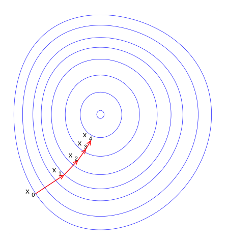
In gradient descent, we begin with a guess \(x^{(0)}\) and a step size \(\gamma > 0\). We proceed iteratively: for each iteration \(i = 1, \dots, K\), let \[ x^{(i)} = x^{(i - 1)} - \gamma \nabla f\left(x^{(i - 1)}\right). \] Stop when the sequence converges or we reach a set maximum number of iterations.
The intuition is straightforward, though it hides some complexity. We can think of the gradient \(\nabla f(x^{(i - 1)}) \in \R^p\) as giving the direction in which \(f(x)\) increases most steeply, so the negative of this is the opposite direction, in which \(f(x)\) decreases most steeply. We move a step in this direction and try again. If our steps are of reasonable sizes, we will tend to move downhill, finding progressively smaller values of the function.
The hidden complexity is the choice of the step size \(\gamma\) and the behavior of gradient descent when \(f\) has a complicated shape, potentially with multiple maxima, minima, and inflection points. You’ll explore some of this behavior on your homework.