15  The Bootstrap

\[ \DeclareMathOperator{\E}{\mathbb{E}} \DeclareMathOperator{\R}{\mathbb{R}} \DeclareMathOperator{\var}{Var} \DeclareMathOperator{\ind}{\mathbb{1}} \]

Note

This chapter is based partly on notes cowritten with Ann Lee and Mark Schervish for 36-402, themselves based in part by notes by Cosma Shalizi.

So far, when we have discussed inference (such as hypothesis tests and confidence intervals), we have used it to try to learn about the underlying population relationships, such as to do inference on the factors associated with some outcome. To do this inference, we relied on mathematical derivations of the distribution of estimators and statistics. These derivations rely on certain assumptions about the data and the population it is drawn from, and if those assumptions are not true, the derivations are not valid. This poses a problem if we want to model poorly behaved data. In this chapter, we’ll discuss a much more general procedure to estimate the distribution of estimators and statistics.

In very generic terms, we can think of the statistical inference process as:

1. We obtain data \(X_1, X_2, \dots, X_N \sim F\), where \(F\) is an unknown population distribution.
2. We calculate \(T = g(X_1, X_2, \dots, X_N)\), some statistic of interest. If we assume \(F\) is a distribution from some parametric family, \(T\) may be an estimator \(\hat \theta\) of the parameter \(\theta\) of that distribution. Because \(T\) is a function of the random sample, it is a random variable.
3. To produce confidence intervals or tests, we want to know \(\var(T)\), which is the variance of \(T\) upon drawing repeated random samples of size \(N\) from \(F\). Or, depending on the situation, we may want to know the entire sampling distribution of \(T\).

We have previously achieved this in two ways:

1. Direct calculation. In Theorem 5.3, for instance, we obtained \(\var(\hat \beta)\) for the OLS estimator by deriving its variance from a basic assumption about \(\var(e \mid X)\).
2. Large-sample approximation. For example, Theorem 11.2 describes the asymptotic distribution of the likelihood ratio test statistic as \(N \to \infty\); in finite samples, this is an approximation, but we can still use it to obtain approximate tests and confidence intervals.

But we often cannot use either approach. We might not believe the assumptions necessary for direct calculation, or our diagnostics may have given reason to doubt them; we might be using an estimator for which we do not know how to do the math; or the approximations necessary may turn out to be too approximate.

This is where the bootstrap comes in. The bootstrap is a general procedure to estimate the distribution of estimators and statistics. It still requires some conditions of the estimator and the data, but far fewer than our previous approaches, and is easy to implement without any complicated math.

15.1 The bootstrap procedure

Before we discuss the bootstrap for regression, let’s consider inference for a statistic \(T\), as above. We’ll then extend our results to regression.

The basic idea of the bootstrap comes from putting two simple ideas together. First: If it were possible to obtain \(B\) repeated samples \(X_1, X_2, \dots, X_N \sim F\), calculating \(T_1, T_2, \dots, T_B\), we could estimate \(\var(T)\) by calculating the sample variance of \(T_1, T_2, \dots, T_B\). We could similarly estimate any other property of the distribution of \(T\) by obtaining enough samples and estimating it.

Of course, the problem is we can’t obtain \(B\) repeated samples from \(F\). That’s why the second idea is also necessary. We do not know \(F\), but we have \(N\) samples from it. If \(F(x)\) is the cumulative distribution function (cdf), we can approximate the cdf by its empirical version, and we can draw new samples from this approximation of the population distribution \(F\).

Definition 15.1 (Empirical cdf) If \(X_1, X_2, \dots, X_N \sim F\), where \(F\) is an unknown distribution with cdf \(F(x)\), then the empirical cdf is \[ \hat F(x) = \frac{1}{N} \sum_{i=1}^N \ind(X_i \leq x), \] where \(\ind(\cdot)\) is the indicator function that is 1 if its argument is true and 0 otherwise.

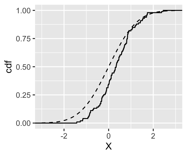
Example 15.1 Suppose \(F\) is the standard normal distribution and \(N = 100\). Figure 15.1 shows the empirical cdf calculated from such a sample, compared to the true standard normal cdf. The empirical cdf matches quite closely.

Figure 15.1: The empirical cdf of 100 draws from the standard normal distribution, compared to the true cdf.

To draw samples from \(\hat F\), it is sufficient to draw samples with replacement from \(X_1, X_2, \dots, X_N\). This leads to the bootstrap procedure.

Definition 15.2 (The bootstrap) Given a sample \(X_1, X_2, \dots, X_N\) from an unknown distribution \(F\), and a statistic \(T = g(X_1, X_2, \dots, X_N)\), the bootstrap estimate of \(\var(T)\) is obtained by the following steps:

1. Estimate \(\hat F\) using the empirical cdf.
2. Draw \(X_1^*, X_2^*, \dots, X_N^* \sim \hat F\).
3. Compute \(T^* = g(X_1^*, X_2^*, \dots, X_N^*)\).
4. Repeat steps 2 and 3 \(B\) times, to get \(T_1^*, T_2^*, \dots, T_B^*\).
5. Let \[ \widehat{\var}(T) = \frac{1}{B} \sum_{b=1}^B \left(T_b^* - \frac{1}{B} \sum_{r = 1}^B T_r^*\right)^2, \] the sample variance of \(T_1^*, \dots, T_B^*\).

We can think of this procedure as making two approximations:

1. We use \(\hat F \approx F\) to approximate drawing from the population distribution. This approximation’s quality depends on \(N\).
2. We approximate the variance of \(T\) using only \(B\) bootstrap samples. We can make this error small by making \(B\) large, unless it is too computationally intensive to do so.

For more details on the error inherent in the bootstrap, see Davison and Hinkley (1997), section 2.5.2. For a discussion of the technical conditions under which bootstrap methods work and don’t work, see Davison and Hinkley (1997), section 2.6.

15.2 Bootstrap confidence intervals

A common application of the bootstrap is the construction of confidence intervals. A \(1 - \alpha\) confidence interval for a parameter \(\theta\) is defined as an interval \([L, U]\) such that \[ \Pr(L \leq \theta \leq U) = 1 - \alpha. \] Here \(L\) and \(U\) are random, because they are calculated from the random data; \(\theta\) is a fixed population parameter. The probability, then, is over repeated resampling of the population, and says that a procedure for generating 95% confidence intervals should produce intervals that cover the population parameter 95% of the time.

We can use the bootstrap to obtain confidence intervals.

Theorem 15.1 (Pivotal bootstrap confidence intervals) If \(X_1, X_2, \dots, X_N \sim F\), and we are interested in estimating a population parameter \(\theta\), we can use the bootstrap to obtain \(\hat \theta_1^*, \hat \theta_2^*, \dots, \hat \theta_B^*\). Then a \(1 - \alpha\) bootstrap confidence interval for \(\theta\) is the interval \[ [2 \hat \theta - q_{1 - \alpha/2}, 2\hat \theta - q_{\alpha/2}], \] where \(\hat \theta\) is the estimate calculated from the sample \(X_1, X_2, \dots, X_N\), and \(q_\alpha\) is the \(\alpha\) quantile of the bootstrap estimates \(\hat \theta_b^*\).

This interval is first-order accurate, meaning \(\Pr(L \leq \theta \leq U) = 1 - \alpha + O(N^{-1/2})\).

Proof. By definition of the quantiles, we have: \[\begin{align*} 1 - \alpha &= \Pr\left(q_{\alpha/2} \leq \hat \theta^* \leq q_{1 - \alpha/2}\right)\\ &= \Pr\left(q_{\alpha/2} - \hat{\theta} \leq \hat \theta^* - \hat{\theta} \leq q_{1-\alpha/2} - \hat{\theta} \right). \end{align*}\] Here \(\hat \theta\) is fixed (to the value obtained from our sample) and \(\hat \theta^*\) is a random variable, since it is obtained from random bootstrap samples. If the distribution of \(\hat \theta - \theta\) (where \(\theta\) is fixed and \(\hat \theta\) is random) is approximately equal to the distribution of \(\hat \theta^* - \hat \theta\), then \[\begin{align*} 1 - \alpha &\approx \Pr\left(q_{\alpha/2} - \hat \theta \leq \hat \theta - \theta \leq q_{1 - \alpha/2} - \hat \theta\right)\\ &= \Pr\left(q_{\alpha/2} - 2 \hat \theta \leq - \theta \leq q_{1 - \alpha/2} - 2 \hat \theta\right)\\ &= \Pr\left(2 \hat \theta - q_{1 - \alpha/2} \leq \theta \leq 2 \hat \theta - q_{\alpha/2}\right). \end{align*}\]

To establish the accuracy of the interval, see Davison and Hinkley (1997), section 5.4.1.

There are in fact many variations of procedures for producing bootstrap confidence intervals, each with different asymptotic properties. Some of these have coverage probability \(1 - \alpha + O(N^{-1})\), which is better than the pivotal intervals described above. For detailed discussion, see Davison and Hinkley (1997), chapter 5.

More recently, specialized (and more computationally intensive) bootstrap confidence interval methods for linear regression have been developed. One recent method, which achieves coverage probability \(1 - \alpha + O(N^{-2})\), is given by McCarthy et al. (2018).

15.3 Resampling cases in regression

Now that we know a general procedure for inference and confidence intervals, let’s apply it to regression. In regression, we obtain samples \(X, Y \sim F\), where \(F\) is an unknown population distribution; we often condition on \(X\), but that is not necessary. To bootstrap, we need a way to simulate new data \((X_1^*, Y_1^*), \dots, (X_N^*, Y_N^*)\) from an approximation of \(F\).

There are many options available, depending on assumptions are willing to make. For example, if our regression model is \(Y = r(X) + e\), for some function \(r\) (such as a linear function), we might trust our estimate \(\hat r(X)\), fix \(X\), and draw new errors to obtain \(Y^*\). But in this course we will introduce only the most general bootstrap for regression: the x-y bootstrap, also known as resampling cases, or just “the” bootstrap.

This bootstrap works in exactly the same way as the bootstrap in the univariate case. It may seem less obvious how to define an empirical cdf \(F(x, y)\) for data where \(X \in \R^p\), but it is still true that drawing \((X, Y)\) pairs with replacement from the sample is the same as drawing from the empirical distribution \(\hat F\).

Definition 15.3 (The x-y bootstrap) Given a sample \((X_1, Y_1), (X_2, Y_2), \dots, (X_N, Y_N)\) from an unknown distribution \(F\), and a statistic \(T\) calculated from this sample, the x-y bootstrap estimate of \(\var(T)\) is obtained by the following steps:

1. Draw \((X_1^*, Y_1^*), (X_2^*, Y_2^*), \dots, (X_N^*, Y_N^*)\) by sampling \(N\) observations with replacement from the data.
2. Compute \(T\), the statistic of interest.
3. Repeat steps 1 and 2 \(B\) times, to get \(T_1^*, T_2^*, \dots, T_B^*\).
4. Let \[ \widehat{\var}(T) = \frac{1}{B} \sum_{b=1}^B \left(T_b^* - \frac{1}{B} \sum_{r = 1}^B T_r^*\right)^2, \] the sample variance of \(T_1^*, \dots, T_B^*\).

Here \(T\) could be a coefficient from a particular model fit to the data; for instance, \(T\) could be \(\hat \beta_1\), and estimating its variance could help us calculate a standard error; or we could use the bootstrap samples to calculate a pivotal confidence interval following the procedure of Theorem 15.1.

Example 15.2 (Bootstrapping with rsample) The rsample package is meant to make it easy to do bootstrap sampling, as well as to do cross-validation (which we will see later). We will use it for all our bootstrapping.¹

Let’s consider the cats data from Exercise 7.1. Let’s again consider predicting heart weight from body weight:

library(MASS)
library(dplyr)
library(rsample)

cat_fit <- lm(Hwt ~ Bwt, data = cats)

Let’s try to obtain a 95% confidence interval for the Bwt coefficient. To do so, we can obtain \(B = 1000\) bootstrap samples from the original data frame, each by drawing \(N = 144\) observations with replacement from the cats data frame (which has 144 rows). The bootstraps() function automatically does resampling with replacement from a dataframe:

boot_samps <- bootstraps(cats, times = 1000)
head(boot_samps)

# A tibble: 6 × 2
  splits           id           
  <list>           <chr>        
1 <split [144/53]> Bootstrap0001
2 <split [144/51]> Bootstrap0002
3 <split [144/52]> Bootstrap0003
4 <split [144/53]> Bootstrap0004
5 <split [144/48]> Bootstrap0005
6 <split [144/54]> Bootstrap0006

boot_samps is now a data frame containing 1000 rows, each of which has a label (id) and an object containing the resampled data. (This is called splits because the package also does cross-validation, where we split the data into training and test sets.)

To finish the bootstrap procedure, we need to refit the model to each of the 1000 bootstrap samples and obtain the Bwt coefficient from each fit. We can use sapply to call a function with each bootstrap sample. Within that function, we call analysis() to get the analysis set (the data to fit the model to) from the object bootstraps() created, and then we can fit a model and get the coefficient.

bwts <- sapply(boot_samps$splits, function(sample) {
  boot_data <- analysis(sample)

  boot_fit <- lm(Hwt ~ Bwt, data = boot_data)

  return(coef(boot_fit)["Bwt"])
})

bwts is now a vector of 1000 coefficients from our 1000 bootstrap samples. Its sample standard deviation is

sd(bwts)

[1] 0.3131108

This is a bootstrap estimate of the standard error. This is larger than the estimate using Theorem 5.3, which is \(0.25\).

We can then apply Theorem 15.1 to obtain a 95% confidence interval for the Bwt coefficient:

2 * coef(cat_fit)["Bwt"] - quantile(bwts, c(0.975, 0.025),
                                    names = FALSE)

[1] 3.408739 4.641188

Compare that to the value calculated by R based on the \(t\) distribution procedure in Section 5.3.1:

confint(cat_fit)["Bwt", ]

   2.5 %   97.5 % 
3.539343 4.528782 

The bootstrap interval is slightly wider.

You can think of a template for bootstrapping regression. If you want to bootstrap \(T\), some statistic calculated from the model, then:

1. Use rsample’s bootstraps() to obtain the bootstrap samples \(b = 1, \dots, B\). Typically \(B = 1000\) or larger.
2. Write a function that fits your desired model to a sample \(b\) and extracts \(T_b^*\).
3. Apply that function to each bootstrap sample. You can use sapply, or if you’re already familiar with the purrr package, you can use any of its map family of functions.
4. Using \(T_1^*, T_2^*, \dots, T_B^*\), calculate your bootstrap standard error, confidence interval, or any other desired quantity.

The same procedure can be applied to ordinary linear models, to any generalized linear model, or to any model based on an iid sample from a population \(F\). (If the sample is not iid, then resampling from the observed data is not like obtaining a sample from the population.)

15.4 Exercises

Exercise 15.1 (Width of bootstrap confidence intervals) In Exercise 9.4, you simulated data for linear regression with heteroskedastic errors. Specifically, the variance of the errors was proportional to \(X_2 / 10\).

1. Consider estimating \(\E[Y \mid X_1 = 5, X_2 = 1]\) using linear regression. Produce a confidence interval using predict() and its interval argument, then produce a pivotal bootstrap confidence interval.

2. Now consider estimating \(\E[Y \mid X_1 = 5, X_2 = 9]\). Again produce a confidence interval using standard errors from predict() and a separate pivotal bootstrap confidence interval.

3. You should see that in one case, the standard interval is wider, but in the other case the bootstrap interval is wider. Explain why.

   Hint: The difference between these two predictions is \(X_2\). This means \(\var(Y \mid X_1 = x_1, X_2 = x_2)\) is different as well.

Exercise 15.2 (Inheritance of height redux) In Exercise 7.2, you related the heights of mothers and their adult daughters to study the inheritance of height. Repeat your regression from that problem and find a pivotal bootstrap confidence interval for the mheight coefficient.

Exercise 15.3 (Insect attraction to light, redux) In Exercise 13.5, you used a generalized linear model to model the number of insects collected in light traps as a function of light type, location, temperature, humidity, and moon phase. In part 4, you gave a 95% confidence interval for the coefficient for temperature.

1. Produce a 95% pivotal bootstrap confidence interval for the same coefficient.
2. Comment on the difference between this confidence interval and the original one. Your original CI was based on an asymptotic result (either the Wald intervals, based on asymptotic normality, or profile likelihood intervals, based on the asymptotic distribution of the likelihood ratio statistic), so it was not exact. (See Section 12.5.2.)

Exercise 15.4 (Bootstrapping the GMP data) TODO HW8 #2 (d)

Davison, A. C., and D. V. Hinkley. 1997. Bootstrap Methods and Their Application. Cambridge University Press.

McCarthy, Daniel, Kai Zhang, Lawrence D. Brown, Richard Berk, Andreas Buja, Edward I. George, and Linda Zhao. 2018. “Calibrated Percentile Double Bootstrap for Robust Linear Regression Inference.” Statistica Sinica 28: 2565–89. https://doi.org/10.5705/ss.202016.0546.

---

1. The boot package is designed specifically for bootstrapping and supports doing bootstrap calculations in parallel, but it is much more complicated than we need here—it supports many varieties of bootstrap sampling we will not be using.