2 Causality
\[ \DeclareMathOperator{\E}{\mathbb{E}} \DeclareMathOperator{\R}{\mathbb{R}} \DeclareMathOperator{\RSS}{RSS} \DeclareMathOperator{\AIC}{AIC} \DeclareMathOperator{\bias}{bias} \DeclareMathOperator{\MSE}{MSE} \DeclareMathOperator{\VIF}{VIF} \DeclareMathOperator{\var}{Var} \DeclareMathOperator{\cov}{Cov} \DeclareMathOperator{\cor}{Cor} \DeclareMathOperator{\se}{se} \DeclareMathOperator{\trace}{trace} \DeclareMathOperator{\vspan}{span} \DeclareMathOperator{\proj}{proj} \newcommand{\condset}{\mathcal{Z}} \DeclareMathOperator{\cdo}{do} \newcommand{\ind}{\mathbb{I}} \newcommand{\T}{^\mathsf{T}} \newcommand{\X}{\mathbf{X}} \newcommand{\Y}{\mathbf{Y}} \newcommand{\Z}{\mathbf{Z}} \newcommand{\zerovec}{\mathbf{0}} \newcommand{\onevec}{\mathbf{1}} \newcommand{\trainset}{\mathcal{T}} \DeclareMathOperator*{\argmin}{arg\,min} \DeclareMathOperator*{\argmax}{arg\,max} \DeclareMathOperator{\SD}{SD} \newcommand{\dif}{\mathop{\mathrm{d}\!}} \newcommand{\convd}{\xrightarrow{\mathrm{D}}} \DeclareMathOperator{\logit}{logit} \newcommand{\ilogit}{\logit^{-1}} \DeclareMathOperator{\odds}{odds} \DeclareMathOperator{\dev}{Dev} \DeclareMathOperator{\sign}{sign} \DeclareMathOperator{\normal}{Normal} \DeclareMathOperator{\binomial}{Binomial} \DeclareMathOperator{\bernoulli}{Bernoulli} \DeclareMathOperator{\poisson}{Poisson} \DeclareMathOperator{\multinomial}{Multinomial} \DeclareMathOperator{\uniform}{Uniform} \DeclareMathOperator{\edf}{edf} \]
As you read the research literature and become more familiar with the kinds of questions answered in medicine, biology, the social sciences, public policy, and so on, you will learn that about half of researchers are trying to answer causal questions: questions about how a particular variable causes changes in another variable, or whether it does so at all. The other half of researchers are lying.1
Consequently, we need a formal way of describing causality. What does it mean to say something “causes” something else? And we will need a language to describe our research goals when answering causal questions. When we have numerous variables with complicated relationships, deciding what we are looking for—which variables must be included in a model, what coefficients or tests or predictions will answer the research question, what types of confounding or bias we must worry about—is often harder than conducting the analyses. Having a formal way to describe our goals will give us a formal way to reason about them.
There are two dominant frameworks used by statisticians to talk about causality: the potential outcomes framework, which provides a definition of “causality” and a way of reasoning about it mathematically, and causal diagrams, which provide a great way to illustrate causal relationships graphically and to reason about our models. We’ll start with counterfactuals, but we will mainly use causal diagrams in this course, simply because they let us sketch out regression problems and reason about how we might estimate the causal effects we want.
2.1 Counterfactuals
2.1.1 Definitions
Let’s start with some notation. Suppose our dataset consists of \(n\) patients, subjects, or units, indexed with \(i = 1, \dots, n\). We are interested in how a particular treatment causes a particular outcome. For simplicity, we’ll suppose there are only two possible treatments, coded as 0 and 1, where 1 is a treatment and 0 is a control. We let: \[\begin{align*} Z_i &= \text{treatment assignment (0 or 1)} \\ X_i &= \text{vector of covariates} \\ U_i &= \text{vector of unobserved covariates.} \end{align*}\] The treatment assignment \(Z_i\) might be within our control (in a randomized experiment) or might be out of our control (in an observational study). \(X_i\) contains other observed covariates that may affect the patient’s outcome, while \(U_i\) encapsulates all the unknown features of the patient that may also affect their outcome.
With these defined, we can define potential outcomes. The potential outcomes give the value of the outcome if the patient were to receive a particular treatment: \[\begin{align*} C_i(1) &= \text{potential outcome of $i$ under treatment ($Z_i = 1$)} \\ C_i(0) &= \text{potential outcome of $i$ under control ($Z_i = 0$)} \\ (C_i(0), C_i(1)) &= \text{causal effect} \\ Y_i &= C_i(Z_i) = \text{observed outcome.} \end{align*}\]
We call \(C_i(0)\) and \(C_i(1)\) the potential outcomes because they are exactly that: potential. They are hypothetical variables representing what would happen if a particular person received a particular treatment, holding everything else (including \(X_i\) and \(U_i\)) fixed. In a particular study, a person may only receive one treatment and not both, and so we only observe \(Y_i = C_i(Z_i)\)—we cannot know both \(C_i(0)\) and \(C_i(1)\).2 We don’t have the convenience of simply loading up a data frame with the potential outcomes and running an analysis.
Example 2.1 (Fixitol and Solvix) To determine whether the new drug Fixitol is more effective than the old medication Solvix for treating malaise, we will examine patients with malaise with the Malaise Measurement Meter after they are treated. Fixitol is better if it reduces malaise scores more than Solvix does. We’ll call Fixitol the treatment and Solvix the control.
However, we also know that other factors affect malaise, such as the amount of sunlight a person gets, their age, other medications they might be taking, and even their ketchup consumption. (Ketchup has natural mellowing agents that reduce malaise.) We can measure some of these factors, but others may be difficult to measure, or we may not even know we need to measure them because we don’t fully understand malaise and everything related to it.
In this case:
- \(Z_i\) indicates if person \(i\) received Fixitol or Solvix to treat their malaise
- \(X_i\) might be a vector giving their ketchup consumption, age, and other demographic variables
- \(U_i\) is an unknown and unobserved vector of everything else that might be related to malaise
- \(C_i(1)\) is the malaise score that person \(i\) would receive if they took Fixitol, while \(C_i(0)\) is the malaise score person \(i\) would receive if they took Solvix.
Potential outcomes let us define causality. A treatment causes a change in outcome for person \(i\) if \(C_i(0) \neq C_i(1)\), holding fixed all other attributes \(X_i\) and \(U_i\) of that person. In Example 2.1, Fixitol causes an improvement relative to Solvix if \(C_i(1) < C_i(0)\): your malaise after taking Fixitol would be less than your malaise after taking Solvix.
2.1.2 Estimating counterfactuals
Because counterfactuals are essentially unobservable (unless you have a time machine, or a particularly niche experimental setup in which you can give multiple treatments to each subject without them interacting with each other), we can’t actually estimate both \(C_i(0)\) and \(C_i(1)\) from data for each \(i\). But we might be interested in averages: can we estimate \(\E[C_i(0)]\) and \(\E[C_i(1)]\)?
Of course. You can take entire courses on sophisticated methods that apply in particular situations. But a very simple approach might be to ask: Can we draw a random sample from the populations of \(C_i(0)\) and \(C_i(1)\)? If so, we can estimate their expectations with sample means. If they are true random samples, these will be unbiased, and the law of large numbers will be on our side.
How do we obtain a random sample? If we have \(n\) people in our study, take half at random. For that half, obtain \(C_i(1)\)—that is, assign them to take the treatment, and ensure they do. For the other half, obtain \(C_i(0)\) by assigning them to take the control. Measure the outcome variable.
This is random assignment, the simplest and perhaps most effective way to estimate potential outcomes. Without random assignment, the estimation problem is much more challenging. Consider that \(C_i(0)\) and \(C_i(1)\) may depend on the covariates \(X_i\) and the unobserved covariates \(U_i\). If the treatment assignment \(Z_i\) also depends on these covariates—if people with certain covariates are more or less likely to get the treatment—then we observe \(C_i(1)\) for a biased sample.
We can try to avoid this problem in various ways. We could, for instance, try to match using the covariates \(X_i\): compare each treated person to a control person with very similar covariates \(X_i\). This would work if there are no important unobserved covariates \(U_i\). We could also try to model the effects of \(X_i\), as we will see later.
In general the estimation of causal effects without random assignment is a complex subject, and there are many specialized methods for specific scenarios that are outside the scope of this course. For more detail, see a book like Hernán and Robins (2020) or Rosenbaum (2020).
2.1.3 Average treatment effects
Using counterfactuals, we can define useful quantities that we may try to estimate using data. For instance, many studies are interested in the average treatment effect.
Definition 2.1 (Average treatment effect) The average treatment effect for a binary treatment is the difference \(\E[C_i(1) - C_i(0)]\).
Counterfactuals are useful for providing these definitions and for doing mathematical analyses of causal estimators. But for reasoning about models for a specific dataset, causal diagrams are very useful.
2.2 Causal diagrams
We can represent causal relationships between variables as directed acyclic graphs (DAGs). Initially, these graphs will only represent dependence between random variables, but later we will see how to describe causal claims using the same graphical language.
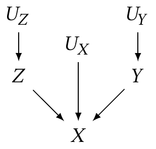
Example 2.2 (A simple DAG) Suppose we have observable random variables \(X\), \(Y\), and \(Z\), and unobservable random variables \(U_X\), \(U_Y\), and \(U_Z\). We can draw a diagram:
This diagram is called a causal graph or causal diagram. Each node represents a random variable in the population.
In a causal diagram, the directed arrows imply dependence: Example 2.2 implies that \[\begin{align*} Z &= f_Z(U_Z) \\ Y &= f_Y(U_Y) \\ X &= f_X(Y, Z, U_X), \end{align*}\] and the \(U\) variables are drawn from their own joint distribution. The form of these functions is unspecified by the diagram: they need not be linear, \(f_X\) need not be separable into components by variable, and so on.
We can think of the \(U\) variables as representing the random variation, error, or noise in our system, which is why I called them “unobservable”: in a particular observed dataset, we will have many observations of \(X\), \(Y\), and \(Z\), but not \(U_X\), \(U_Y\), or \(U_Z\). Typically we omit them from the diagrams, because every problem in statistics has noise everywhere, and relationships are very rarely deterministic. When we omit them, we imply they are independent; if two variables in the diagram have sources of error that are dependent, that error source should be explicitly included as a node in the diagram.
Definition 2.2 (Graph terminology) Let’s define graph terminology by using Example 2.2:
- A node or vertex is connected to other nodes by edges. The nodes \(X\) and \(Z\) are connected by an edge from \(Z \to X\), but there is no edge between \(Z\) and \(Y\).
- A directed edge has a direction, represented by an arrow. All edges in causal diagrams are directed edges.
- When an edge goes from one node to another, it starts at the parent node and ends at the child node. This is reflected by the direction of the arrow in the diagram. \(Z\) is a parent of \(X\), and \(X\) is its child.
- A path between two nodes is a route between those two nodes following edges of the graph. For instance, there is a path \(Z \to X \leftarrow Y\).
- A directed path is a path that follows the direction of arrows. There is no directed path from \(Y\) to \(Z\), but there is a directed path from \(U_Z\) to \(X\).
- The descendants of a node are all nodes that can be reached from it by directed paths; the initial node is their ancestor.
- On a path, a collider is a node with two arrows into it. On the path \(Z \to X \leftarrow Y\), \(X\) is a collider. But on the path \(U_Y \to Y \to X\), \(X\) is not a collider.
2.2.1 Conditional independence
Surprisingly, from this simple interpretation of causal graphs as defining functional relationships, we can extract statements about conditional independence of the random variables. We can determine conditional independence by working from the three basic structures that all causal diagrams are built from:
- Chains: Directed paths \(X \to Y \to Z\).
- Forks: \(X \leftarrow Y \to Z\).
- Colliders: \(X \to Y \leftarrow Z\).
These structures determine the dependence in the diagram.
Theorem 2.1 (Dependence in chains) In a chain \(X \to Y \to Z\) (or \(X \to Y\), or \(X \to Y \to \dots \to Z\)), \(X\) and \(Z\) are probably dependent.
However, if we condition on \(Y\), and there is no other path between \(X\) and \(Z\) that could create dependence, then \(X\) and \(Z\) are conditionally independent given \(Y\).
Proof. If there is a directed path from \(X\) to \(Z\), then \(Z\) is a function of \(X\) or of variables that are themselves functions of \(X\): \(Z = f_Z(X, \dots)\) or \(Z = f_Z(f_{\cdot}(\cdots(X)))\). Whatever form those functions takes dictates the relationship between \(X\) and \(Z\). It’s possible in special cases for those functions to produce no relationship between \(X\) and \(Z\), but in most cases they’ll be dependent.
If we condition on \(Y = y\) and there are no other paths between \(X\) and \(Z\) creating dependence, then for simplicity, let’s say the diagram implies \[\begin{align*} X &= f_X(U_X) \\ Y &= f_Y(X, U_Y)\\ Z &= f_Z(Y, U_Z). \end{align*}\] Substituting these together, \[ Z = f_Z(f_Y(X, U_Y), U_Z), \] and so \(Z\) depends on \(X\) in some potentially complicated way. But if we condition on \(Y = y\), then \[ Z = f_Z(y, U_Z), \] and the only source of variation in \(Z\) is \(U_Z\), which is independent noise. There is no longer any relationship to \(X\).
Theorem 2.2 (Dependence in forks) In a fork \(X \leftarrow Y \to Z\) (or \(X \leftarrow \dots \leftarrow Y \to \dots \to Z\)), \(X\) and \(Z\) are probably dependent.
Proof. Both \(X\) and \(Z\) can be written as functions of \(Y\), and so as \(Y\) varies, both \(X\) and \(Z\) vary together, making them dependent.
Theorem 2.3 (Dependence in colliders) In a collider \(X \to Y \leftarrow Z\), if there is no other path between \(X\) and \(Z\) creating dependence, they are independent; however, \(X\) and \(Z\) are dependent when we condition on \(Y\).
Proof. If there are no other paths creating dependence between \(X\) and \(Z\), the collider implies that \[\begin{align*} X &= f_X(U_x)\\ Z &= f_Z(U_z)\\ Y &= f_Y(X, Z, u_Y). \end{align*}\] The random variables \(X\) and \(Z\) are functions of independent noise sources (\(U_X\) and \(U_Z\)), so as written, they are independent. But if we condition on \(Y = y\), then \(f_Y(X, Z, u_Y)\) must be equal to \(y\), and so \(X\) and \(Z\) must have values such that \(f_Y(X, Z, u_Y) = y\). For example, if \[ f_Y(X, Z, U_Y) = 2X - 3Z + u_Y, \] then when we condition on \(Y = y\), \[ 3Z + y = 2X + U_Y, \] and so \(Z\) and \(X\) are linearly correlated.
These three cases are the only way to create dependence in causal diagrams: if none applies, then the variables in question are independent. For instance, two variables with no paths between them at all are always independent—neither can be written as a function of the other. If there is a chain or a fork, they are probably dependent.
Example 2.3 (“Probably” dependent) In the rules above, we said that under certain conditions, \(X\) and \(Z\) are probably dependent. Why probably and not certainly?
Consider a fork \(X \leftarrow Y \to Z\). Let \(Y \sim \normal(0, 1)\). We can define \(X\) and \(Z\) such that they are functions of \(Z\), but independent: \[ X = |Y|, \qquad Z = \frac{Y}{|Y|}. \] Now \(X\) has a folded normal distribution (and hence always positive) and \(Z \in \{-1, 1\}\) is the sign of \(Y\). Because the standard normal distribution is symmetric around 0, the magnitude (\(X\)) is independent of the sign (\(Z\)). Thus \(X\) and \(Z\) are independent.
So it is possible, in certain special cases, to have a fork without dependence. We can concoct other pathological examples for chains. Generally, however, these pathological examples do not occur outside textbook examples.
We can apply these rules of dependence and independence to the joint and conditional distributions of the random variables in the diagrams.
Example 2.4 (Chain of dependence) Consider this causal diagram:
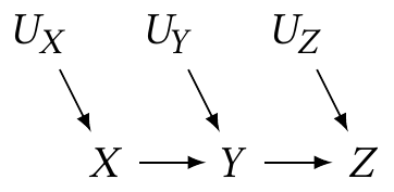
From this diagram, we deduce \[ \Pr(Z = z \mid X = x, Y = y) = \Pr(Z = z \mid Y = y), \] i.e. conditioning on \(Y\) makes \(X\) independent of \(Z\). If we do not condition on \(Y\), we know \(Z\) and \(X\) are likely dependent, because they are in a chain.
Contrast this with Example 2.2. In that DAG, \[ \Pr(Z = z \mid X = x, Y = y) \neq \Pr(Z = z \mid X = x) \] because \(X\) is not a parent of \(Z\). In fact, conditioning on \(X\) makes \(Z\) dependent on \(Y\) when it was not dependent previously. This means \(X\) is a collider on the path \(Z \to X \leftarrow Y\).
Example 2.5 (Berkson’s Paradox) Berkson (1946) first described colliders before causal diagrams had been invented as a way to describe dependence. Suppose we want to know if diabetes is a cause of cholecystitis, an inflammation of the gallbladder. We examine the records of numerous hospital patients and record whether they have diabetes, cholecystitis, or both. This gives us the following causal diagram:
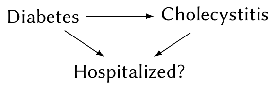
We want to know if the \(\text{diabetes} \to \text{cholecystitis}\) arrow is present. Notice the indicator of whether the person is hospitalized. By using only records of hospital patients, we are conditioning on this variable. This induces dependence between diabetes and cholecystitis even if there is no causal arrow between them: If you are hospitalized, there is presumably a good reason for it; people without diabetes must have some other reason for being hospitalized, making them more likely than average to have cholecystitis. This results in an apparent negative relationship between diabetes and cholecystitis, as Berkson noticed in real hospital records.
Together, Theorem 2.1, Theorem 2.2, and Theorem 2.3 imply conditional independence rules that allow us to decompose the joint distribution of any causal diagram.
Theorem 2.4 (Conditional independence in a causal diagram) The joint distribution of all variables in a causal diagram can be decomposed as \[ \Pr(\text{variables}) = \prod \Pr(\text{child node} \mid \text{parents}). \]
We will “prove” this by example.
Example 2.6 (“Proof”) Consider the diagram shown in Example 2.4. By the definition of conditional probability, \[ \Pr(X, Y, Z, U_X, U_Y, U_Z) = \Pr(Z \mid X, Y, U_X, U_Y, U_Z) \Pr(X, Y, U_X, U_Y, U_Z). \] By Theorem 2.1, \(Z\) is independent of \(X\), \(U_X\), and \(U_Y\) given \(Y\), so this simplifies to \[ \Pr(X, Y, Z, U_X, U_Y, U_Z) = \Pr(Z \mid Y, U_Z) \Pr(X, Y, U_X, U_Y, U_Z). \] We can repeat the same decomposition on \(\Pr(X, Y, U_X, U_Y, U_Z)\): \[ \Pr(X, Y, U_X, U_Y, U_Z) = \Pr(Y \mid X, U_Y) \Pr(X, U_X, U_Y). \] And we can repeat this for each joint distribution in turn, yielding \[\begin{multline*} \Pr(X, Y, Z, U_X, U_Y, U_Z) = \\ \Pr(Z \mid Y, U_Z) \Pr(Y \mid X, U_Y) \Pr(X \mid U_X) \Pr(U_X) \Pr(U_Y) \Pr(U_Z), \end{multline*}\] the product of nodes given their parents.
Because of these properties, if we are interested in a particular relationship—say, \(\Pr(X \mid U_X, Y, Z)\)—we need not estimate the full joint distribution. We can estimate the conditional distribution of interest alone.
We can also use these properties to detect dependence and independence in larger causal graphs containing many chains, forks, and colliders, such as diagrams representing real situations of interest to us.
2.2.2 d-separation
Given an arbitrarily complicated causal graph, and if we condition on an arbitrary collection of random variables in that graph, how can we tell if two selected variables would be statistically dependent or independent? The criterion we use is d-separation (d for “directional”), which extends the rules described above into a formal criterion that can check the dependence of any two nodes in a causal diagram.
Two d-separated variables are independent; d-connected variables are usually dependent. But d-separation depends on conditioning: if we condition on some variables (i.e. hold their value fixed), that changes which variables are d-separated.
Definition 2.3 (d-separation) Consider two nodes \(X\) and \(Y\) in a causal diagram, and every path \(p\) connecting them. (These need not be directed paths.) Suppose we condition on a set of nodes \(\condset\).
\(X\) and \(Y\) are d-separated (when conditioning on \(\condset\)) if all paths \(p\) are blocked. A path \(p\) is blocked by \(\condset\) if and only if
- \(p\) contains a chain \(A \to B \to C\) or fork \(A \leftarrow B \to C\) where \(B \in \condset\), or
- \(p\) contains a collider \(A \to B \leftarrow C\) where \(B \notin \condset\), and no descendant of \(B\) is in \(\condset\).
If \(X\) and \(Y\) are not d-separated, they are d-connected.
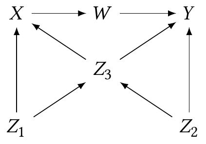
Example 2.7 (d-separation demo) Consider the following causal diagram (Pearl et al. 2016, fig. 2.9):
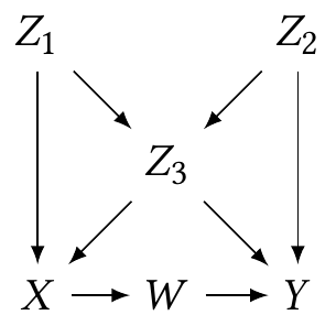
- No conditioning. \(W\) and \(Z_2\) are d-connected. The path \(Z_2 \to Z_3 \to X \to W\) is not blocked. But \(Z_1\) and \(Z_2\) are d-separated, because all possible paths between them contain a collider that is not conditioned on (such as \(Z_3\) in the path \(Z_1 \to Z_3 \leftarrow Z_2\)).
- Condition on \(Z_3\). \(W\) and \(Z_2\) are still not d-separated. The \(Z_2 \to Y \leftarrow W\) path is blocked, because it has a collider (\(Y\)) that is not conditioned on; the path \(Z_2 \to Z_3 \to X \to W\) is a chain blocked by conditioning on \(Z_3\). But the \(Z_2 \to Z_3 \leftarrow Z_1 \to X \to W\) path is not blocked, because \(Z_3\) is a collider on that path. On the other hand, \(Z_1\) and \(Z_2\) are now connected, because the path \(Z_1 \to Z_3 \leftarrow Z_3\) is not blocked, as the colliding node is conditioned on.
So why do we care about d-separation? First, it means causal diagrams have testable implications: From a diagram we can determine which variables are independent, and if we can test for independence using data, we can test the diagram.3 The field of causal discovery attempts to use tests to determine which causal diagrams are compatible with observed data.
Second, it helps us determine which effects can and cannot be estimated from observed data alone. Let’s consider two examples.
Example 2.8 (No confounding) Suppose patients receive a treatment and we measure an outcome. This outcome is also influenced by a prior condition the patients have, but we do not observe this prior condition. The diagram is:
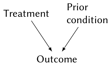
We can estimate \(\Pr(\text{outcome} \mid \text{treatment})\) from data, but we can’t include the prior condition because it is unobserved. By the law of total probability, we are really estimating \[\begin{multline*} \Pr(\text{outcome} \mid \text{treatment}) = \\ \sum_\text{conditions} \Pr(\text{outcome} \mid \text{treatment}, \text{condition}) \Pr(\text{condition} \mid \text{treatment}), \end{multline*}\] and since condition and treatment are d-separated, \(\Pr(\text{condition} \mid \text{treatment}) = \Pr(\text{condition})\). Hence the association in observed data is the average relationship between treatment and outcome, averaging over prior conditions based on their prevalence.
We can thus estimate the association between treatment and outcome using only the observed variables.
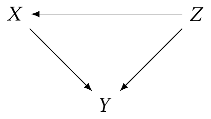
Example 2.9 (Confounding) On the other hand, suppose that the prior condition influences the treatment and outcome, but the treatment has no effect on the outcome whatsoever. For example, maybe doctors tend to treat patients differently based on their prior condition, but haven’t realized the treatments are equivalent:
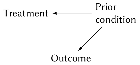
Again, suppose the prior condition is unobserved. We can again write out the law of total probability, but in this case, \(\Pr(\text{condition} \mid \text{treatment}) \neq \Pr(\text{condition})\), while \(\Pr(\text{outcome} \mid \text{treatment}, \text{condition}) = \Pr(\text{outcome} \mid \text{condition})\) because the treatment is ineffective. Consequently, \[\begin{multline*} \Pr(\text{outcome} \mid \text{treatment}) = \\ \sum_\text{conditions} \Pr(\text{outcome} \mid \text{condition}) \Pr(\text{condition} \mid \text{treatment}), \end{multline*}\] and so the distribution of outcomes depends on the treatment, even though the treatment has no causal effect on outcome.
In this case, we say prior condition is a confounding variable, because it creates association between the treatment and outcome even if the treatment does not cause the outcome. Contrast this to Example 2.8, where because the condition caused the outcome but not the treatment, it was not a confounding variable.
These examples illustrate that each path between two nodes in a causal diagram—paths that may be blocked or open based on the d-separation criteria—represents a source of association between those variables, and all other variables on that path may influence the association.
2.2.3 Causal interpretation of DAGs
Because causal diagrams represent deterministic functional relationships between variables (some of which may be random), we can interpret them causally. Any node is a function of its parents, and so if one of its parents is changed, its value changes accordingly. We can directly connect this to the counterfactual definition of causality in Section 2.1, and this applies even if we omit the unobserved noise random variables and consider relationships to be random.
If we are interested in the causal relationship between treatment and outcome, we are implicitly interested in only specific paths: the directed paths from the treatment to the outcome. If there are any other open paths, such as from confounding variables or from colliders we have conditioned on, the observed association between treatment and outcome will be the association from all the paths, not simply the directed causal paths of interest. If we want to estimate the causal effect alone—for example, to know what would happen if we assigned a particular treatment instead of allowing it to be influenced by prior condition—we to isolate the particular causal effect of interest by blocking the undesired paths.
2.2.4 The backdoor criterion
We can isolate a causal path of interest by using d-separation determine how to block all other paths, but this can be laborious in a large causal graph. The backdoor criterion gives us a simpler sufficient condition to determine when those paths have been blocked.
Definition 2.4 (Backdoor criterion) When estimating the causal effect of \(X\) on \(Y\), a set of variables \(\condset\) satisfies the backdoor criterion if no node in \(\condset\) is a descendant of \(X\), and the nodes in \(\condset\) block every path between \(X\) and \(Y\) that contains an arrow into \(X\).
Paths between \(X\) and \(Y\) containing an arrow into \(X\) are called backdoor paths, as they represent confounding or other unwanted association.
The backdoor criterion is a sufficient condition, but not necessary: it is possible to isolate a causal effect in other ways. You can always use d-separation to tell if you have blocked paths other than the paths of interest. But most of the time, when we are simply controlling for confounding variables, we are satisfying the backdoor criterion. It’s only in unusual or creative cases that we identify a causal effect another way.
Example 2.10 Suppose we are examining the causal effect of a particular treatment on recovery, as in Example 2.8. However, we know there is a confounding path (in blue):
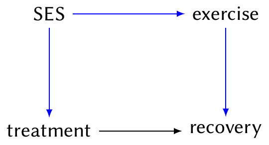
Here SES is socioeconomic status. It causally effects treatment (because some people cannot afford more expensive treatments), and also exercise (because personal trainers are expensive and having time for the gym is related to your job); and recovery from this condition is related to exercise.
The path \(\text{treatment} \leftarrow \text{SES} \to \text{exercise} \to \text{recovery}\) is a backdoor path, because it contains an arrow into treatment.
Suppose we cannot measure SES in this study and hence cannot condition on it. If we can measure and condition on exercise levels, we block the blue path and satisfy the backdoor criterion. Conditioning on exercise is hence sufficient to allow us to identify the causal effect of treatment on recovery.
2.2.5 Graph surgery through random assignment
The first way to isolate causal effects in the presence of confounders is to perform graph surgery: instead of conditioning on variables, simply change the causal diagram so the backdoor criterion is satisfied. In other words, we intervene to assign the value of a particular node in the graph, instead of allowing it to be affected by other random variables.
Example 2.11 (Random assignment) Consider this situation:
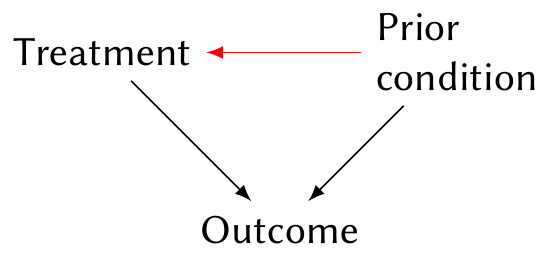
Here prior condition is a confounding variable and may induce association between treatment and outcome even if there is no causal effect. But suppose we flip a coin to randomly assign treatment. Now prior condition has no causal effect on treatment, and so the arrow (in red) from condition to treatment disappears. We are left with no confounding, and can estimate the causal effect from the association between treatment and outcome.
Random assignment is the most robust way to estimate a causal effect; in medicine, randomized clinical trials are known as the gold standard for providing evidence. Random assignment has the advantage of eliminating all possible backdoor paths, even ones we are unaware of: every arrow into the treatment is eliminated. Alternately, we can think of it as balancing all possible confounding variables: because the treatment is randomly assigned, there should be no systematic differences between the treatment groups apart from the treatment we assign.
However, random assignment is not foolproof:
- The causal effect of \(X\) on \(Y\) may not be caused by the reason or mechanism we intended. In a medical trial, for example, if the doctors and nurses in the staff are aware which patients have received which treatment, they may treat the patients differently (intentionally or unintentionally), changing their outcomes. Hence the causal effect of treatment on outcome may involve the behavior of the medical staff, not just the biological effect of the treatment.
- Some random assignment is not so random. We could, for instance, flip a coin and decide that all patients in one hospital will receive one treatment, whereas all patients in another hospital will receive the other treatment. If the hospitals or their patients are systematically different, the effect we measure may be due to the hospital, not the treatment.
- Many randomized experiments involve people, and people are often human. They may not take the treatment, they may not complete the tasks as assigned, or they may not follow instructions.
Random assignment also is not always possible. If I want to study the causal effect of, say, childhood trauma on later life achievement, most authorities would not permit me to randomly assign some children to be traumatized. Similarly, the causal effect of many government policies is difficult to evaluate because governments will not offer to randomly apply the policies to some people and not others.
Example 2.12 (Natural experiments) Sometimes, circumstances provide something like random assignment without an experimenter deliberately assigning treatments. This is called a natural experiment. For example, Kirk (2009) was interested in the causes of recidivism—meaning the causes of re-offense among people convicted of crimes, imprisoned, and then released. One hypothesis was that released prisoners may return to the same neighborhood where they had friends and opportunities that got them into crime, and if they instead live in unfamiliar places without those factors that led them to crime, they may be less likely to reoffend.
However, it is difficult to force released prisoners to live in specific neighborhoods, and presumably their decision of where to live is influenced by many potential confounding factors. But in 2005, Hurricane Katrina hit the coast of Louisiana and destroyed many neighborhoods through floods and wind. Afterwards, some people released from prison could return to their old neighborhoods, but some could not, because their neighborhoods were destroyed. Kirk (2009) used data on prisoners released on parole to conclude that “moving away from former geographic areas substantially lowers a parolee’s likelihood of re-incarceration.”
2.2.6 The do-calculus
The notion of graph surgery through assignment also leads us to a useful concept: the “do-calculus”.
Definition 2.5 (do notation) In the do calculus, we write \(\cdo(X = x)\) to reflect \(X\) being assigned to the value \(x\). For example, \[ \Pr(Y \mid \cdo(X = x)) \] is the conditional distribution of \(Y\) when \(X\) is assigned to be \(x\). This is different from \[ \Pr(Y \mid X = x), \] which is the conditional distribution of \(Y\) for individuals who happen to have the value \(X = x\).
In other words, \(\Pr(Y \mid X = x)\) represents the conditional distribution of \(Y\) in the original causal diagram, and \(\Pr(Y \mid \cdo(X = x))\) represents the conditional distribution of \(Y\) when all arrows into \(X\) are deleted.
We can see the connection to counterfactuals more clearly now. In counterfactual notation, \(Z\) is a treatment assignment and \(C(Z)\) is the counterfactual under that treatment, meaning the potential outcome for each individual if they were assigned that treatment, while \(Y\) is the observed outcome. Here, \(\Pr(Y \mid Z = z)\) is the distribution of observed outcomes among people who get treatment \(z\), while \(\Pr(Y \mid \cdo(Z = z))\) is the distribution of outcomes among people assigned treatment \(z\), and represents those counterfactuals. When we have a binary treatment and binary outcome (such as recovered vs. not recovered), estimating the average treatment effect is the same as estimating \(\Pr(Y = 1 \mid \cdo(Z = 1)) - \Pr(Y = 1 \mid \cdo(Z = 0))\).
Returning to Example 2.11, \(\Pr(\text{outcome} \mid \text{treatment})\) does not represent the causal effect when there is a confounding variable, because \(\Pr(\text{outcome} \mid \text{treatment}) \neq \Pr(\text{outcome} \mid \cdo(\text{treatment}))\). But if we assign the treatment, or otherwise break the confounding path, then \(\Pr(\text{outcome} \mid \text{treatment}) = \Pr(\text{outcome} \mid \cdo(\text{treatment}))\). When we are looking for causal effects, we are looking for ways to estimate the latter.
2.2.7 Adjustment for confounders
Beyond random assignment, the alternative way to isolate causal effects is adjustment. We often hear of studies that “adjust for” or “control for” variables, and these studies are attempting to isolate a causal effect by including variables in the conditioning set \(\condset\).
If we identify a set \(\condset\) that satisfies the backdoor criterion, we can adjust for it using the adjustment formula.
Theorem 2.5 (Adjustment formula) To estimate the causal effect of \(X\) on \(Y\) in a causal diagram, where the set of variables \(\condset\) satisfies the backdoor criterion (Definition 2.4), we can calculate \[ \Pr(Y = y \mid \cdo(X = x)) = \sum_z \Pr(Y = y \mid X = x, \condset = z) \Pr(\condset = z), \] where the sum is over all combinations of values of the variables in the conditioning set \(\condset\). For continuous variables, the sum is replaced with an integral: \[ f_Y(Y = y \mid \cdo(X = x)) = \int f_Y(y \mid X = x, \condset = z) f_Z(z) \dif z. \]
Proof. To derive the adjustment formula, we require several facts about \(\Pr(Y \mid \cdo(X = x))\).
- \(\Pr(Y \mid \cdo(X = x), \condset = z) = \Pr(Y \mid X = x, \condset = z)\), because \(Y\) is the same function of \(X\) and \(Z\) whether we break the \(Z \to X\) arrow or not.
- \(\Pr(\condset = z \mid \cdo(X = x)) = \Pr(\condset = z)\), because \(X\) and \(Z\) are independent when the \(Z \to X\) arrow has been broken by random assignment.
Now we use the law of total probability to write \[\begin{align*} \Pr(Y = y \mid \cdo(X = x)) &= \sum_z \Pr(Y = y \mid \cdo(X = x), \condset = z) \Pr(\condset = z \mid \cdo(X = x)) \\ &= \sum_z \Pr(Y = y \mid \cdo(X = x), \condset = z) \Pr(\condset = z). \end{align*}\] Applying the first fact above produces the adjustment formula.
To calculate or estimate this, we need the values of all the variables in \(\condset\).
Example 2.13 (Adjusting for confounding) In Example 2.8 and Example 2.9, we considered estimating the causal effect of treatment on an outcome when there is a prior condition that could confound the effect. We showed that if the prior condition is a confounder, estimating \(\Pr(\text{outcome} \mid \text{treatment})\) from the data would not estimate the causal effect.
Suppose we can observe the prior condition. Using the adjustment formula, the adjusted effect is \[\begin{multline*} \Pr(\text{outcome} \mid \cdo(\text{treatment})) =\\ \sum_{\text{condition } c} \Pr(\text{outcome} \mid \text{treatment}, \text{condition} = c) \Pr(\text{condition} = c), \end{multline*}\] where the sum is over all the values of the prior condition variable.
Adjustment allows us to estimate causal effects when we cannot randomly assign the treatment. But adjustment’s key weakness is that we must have all the variables in \(\condset\), meaning we must trust that we have included all the variables related to \(X\) and \(Y\) in our causal diagram and we have connected them with the correct set of edges. If there is a confounding variable we are unaware of, or we misunderstand the causal relationship between the variables we are aware of, we may fail to control for all the necessary variables, and our estimate will not be for the correct causal effect.
Just as the backdoor criterion is not the only way to isolate causal effects, adjustment is not the only way to estimate them; there are other approaches that work in different cases. But situations where we can satisfy the backdoor criterion are the most common, and adjustment has a direct connection to the typical regression models we will use, so it’s what we’ll focus on.
Example 2.14 (Kidney stones) Kidney stones are mineral deposits that form in the urinary tract, hardening into small stones. Very small stones can be passed from the body in the urine, but larger stones can get stuck. Anecdotally, kidney stones are extremely painful, often described as worse than childbirth. There are a variety of methods to remove kidney stones, depending on their size and composition.
A 1986 study sought to compare several methods for removing kidney stones (Charig et al. 1986). One method was open surgery, which involves making an incision and physically removing the kidney stone. A newer method was percutaneous nephrolithotomy,4 which uses a much smaller incision to insert a tool to break up the stone so it can be removed in small pieces. The study was observational: it used hospital surgery records that recorded the type of surgery and the outcome. The surgery was defined to be successful if the stones were eliminated or less than 2 mm in size three months after surgery.
| Treatment | Diameter < 2 cm | ≥ 2 cm | Overall |
|---|---|---|---|
| Open surgery | 93% | 73% | 78% |
| Percutaneous nephrolithotomy | 87% | 69% | 83% |
Table 2.1 shows the results of the study. Overall, percutaneous nephrolithotomy had a higher success rate than the more traditional open surgery. But among patients whose kidney stones were smaller than 2 cm, open surgery was more effective—and among patients whose kidney stones were larger, open surgery was also more effective. How could that happen?
The key is that “the probability of having open surgery or percutaneous nephrolithotomy varied according to the diameter of the stones” (Julious and Mullee 1994). Since percutaneous nephrolithotomy was new, surgeons likely chose to use it for simpler cases with smaller stones; and stone size is strongly related to success rate, since larger stones are more difficult to remove. Percutaneous nephrolithomy was used in easier cases than open surgery. Or, in other words, stone size was a confounding variable and the causal diagram looked like this:
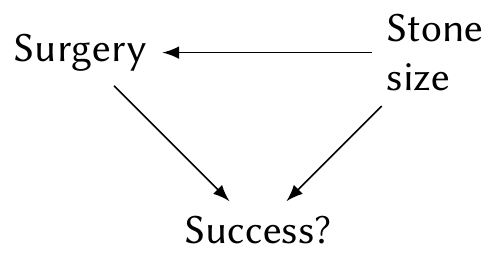
To estimate the causal effect of surgery type on success rate, we need to use the adjustment formula (Exercise 2.3). The paradox exhibited by this data, where an association in the overall dataset reverses when we look within subgroups, is known as Simpson’s paradox.
2.3 Translating questions to causal diagrams
The definitions and rules above describe how we use and interpret causal diagrams, but there is one missing piece. If we’re given a dataset and asked to answer questions about it, how do we know what the correct causal diagram is?
The short answer is “We don’t,” except perhaps in tightly controlled experiments testing precise physical laws. Instead, our analysis is iterative:
- Attempt to understand the data, the variables that have been measured, and how they may be related to each other.
- Attempt to understand the question being asked. Often the question is vague: Which treatment is best? What decision should we make? How do we improve outcomes?
- Sketch a causal diagram linking the known variables. Identify the causal paths of interest, and identify confounding paths that must be blocked.
- Determine what models and methods would be appropriate to answer the questions.
- Apply those models and methods to the data.
- Realize you have misunderstood the problem, the data is unclear, the models don’t work, and there are unexpected confounders. Return to step 1.
- Finally, attempt to communicate the results back to the scientist, policymaker, or client who had the question.
By putting the situation on paper in a simple, easy-to-understand diagram, we can make sure we understand what’s going on, which specific causal effects are of interest, and what models might estimate those effects. Sometimes we discover that the causal effect cannot be estimated, or that some confounding variables cannot be measured or eliminated; sometimes we must tell the scientist their question cannot be answered. The causal diagram and associated methods can help us along the way.
Notice also that the development of the causal diagram is separate from the development of a statistical model. The causal diagram decides how the observable (and unobservable) random variables are related to each other—the true causal diagram is a property of the population, not of the model you choose. Your task is to select a model that matches the questions you want to answer.
2.3.1 Causal diagrams in complex settings
In this iterative data analysis process, step 3 can pose a problem: what if we are evaluating the effect of a government policy, or studying human psychology, or trying to tell if bacon causes cancer? We do not know all the possible variables involved in human psychology and biology, so we only have a vague and incomplete notion of the full causal diagram. Drawing a diagram, even woefully incomplete, may be helpful to organize our thinking, but we may be unable to determine how to estimate our desired causal effect. What can we do?
There are several rules that help us focus our attention on the variables that are most important.
Theorem 2.6 (Pre-treatment variables) A pre-treatment variable is one whose value can be measured before the treatment is assigned or determined. Let \(S\) be the set of all pre-treatment variables. Then \(S\) satisfies the backdoor criterion (Definition 2.4).
Proof. A pre-treatment variable occurs before the treatment, so it cannot be a causal descendant of the treatment. All variables with an arrow into the treatment are pre-treatment. Hence the backdoor criterion is satisfied by definition.
So we do not need to worry about drawing elaborate causal diagrams for post-treatment or post-response variables; we can focus on pre-treatment variables. However, we can refine this criterion further.
Theorem 2.7 (Confounder selection) Let \(S\) be the set of all pre-treatment variables and let \(\operatorname{An}(X)\) denote the set of all ancestors of node \(X\). Then to estimate the causal effect of \(X\) on \(Y\), the set \[ S \cap (\operatorname{An}(X) \cup \operatorname{An}(Y)) \] satisfies the backdoor criterion.
Proof. See VanderWeele and Shpitser (2011).
Hence it is sufficient to find the pre-treatment ancestors of the treatment and the response, and leave all other parts of the causal diagram incomplete. One can extend this rule to cover proxy variables, instrumental variables, and other conditions outside the scope of this course; see VanderWeele (2019).
2.3.2 Recognizing limitations
Of course, we may not even know all pre-treatment ancestors of the treatment and response—some may be unobservable, and some may be true unknown unknowns, causing confounding without our awareness of their existence. A causal diagram represents our knowledge of the situation, and our knowledge is necessarily incomplete. Ultimately we must do the best we can, and acknowledge any limitations in our analysis.
2.4 Connecting causal diagrams to regression models
As defined above, causal diagrams give us ways to describe conditional independence relationships between variables. If we drew a diagram, found the conditional independence relationships, and determined which variables to condition on to find an effect of interest, we could use the observed data to estimate the conditional distributions. But estimating full distributions is difficult—we’d have to use some kind of conditional density estimation, which could require huge amounts of data to do well. In typical statistical practice, we’re more used to estimating expectations: building models to estimate \(\E[Y \mid X]\), for instance.
For example, let’s return to a situation like Example 2.9.
If we want to estimate the causal effect of \(X\) on \(Y\) by conditioning on \(Z\), we can use the adjustment formula (Theorem 2.5), which says that \[ f_Y(Y = y \mid \cdo(X = x)) = \int f_Y(y \mid X = x, Z = z) f_Z(z) \dif z. \] If we instead want the expectation—the expected causal outcome—we have \[\begin{align*} \E[Y \mid \cdo(X = x)] &= \int y f_Y(y \mid \cdo(X = x)) \dif y \\ &= \int_y y \int_z f_Y(y \mid X = x, Z = z) f_Z(z) \dif z \dif y \\ &= \int_z f_Z(z) \int_y y f_Y(y \mid X = x, Z = z) \dif y \dif z \\ &= \int_z \E[Y \mid X, Z] f_Z(z) \dif z \\ &= \E_Z[\E[Y \mid X, Z]], \end{align*}\] where \(\E_Z\) is the expectation with respect to the marginal distribution of \(Z\).
And this is what leads us to regression. A regression model of \(Y\) as a function of \(X\) and \(Z\) is a model that estimates \(\E[Y \mid X, Z]\). If our regression model is good, we identify the right confounding variables \(Z\), and we have sufficient data, we can get a good estimate of \(\E[Y \mid \cdo(X = x)]\). We can then simply average over \(Z\) to obtain the average causal effect of \(X\) on \(Y\).
There are much more sophisticated ways to estimate causal effects, but to start, we’ll use linear regression, with causal diagrams guiding our choice of model.
Exercises
Exercise 2.1 (Causal effect of race) The counterfactual definition of causality has limits. Consider a classic example: Is it possible to define the causal effect of race on, say, socioeconomic status? Is it possible to change race (\(Z_i\)) while holding fixed all variables \(X_i\) and \(U_i\), and if so, does it answer the right question?
Exercise 2.2 (Sample to population) Returning again to Example 2.1, suppose we enroll \(n\) people in our clinical trial. We randomly assign them to take Fixitol or Solvix and measure their malaise afterward. Assuming we measured correctly and people took the medications they were assigned, we now have unbiased estimates of \(C_i(0)\) and \(C_i(1)\) in this population of \(n\) people. Are these necessarily unbiased estimates for the population of all people in the world who have malaise?
Exercise 2.3 (Kidney stone adjustment) The raw data from Example 2.14 is shown in Table 2.2. Again, this is an observational study, and the table shows the number of surgeries that were successful or unsuccessful for stones of different sizes.
| Stone size | Surgery | Successful | Unsuccessful |
|---|---|---|---|
| < 2 cm | Open | 81 | 6 |
| PN | 234 | 36 | |
| ≥ 2 cm | Open | 192 | 71 |
| PN | 55 | 25 |
Using the data in the table, first estimate the unadjusted difference in success rates, \[ \Pr(\text{successful} \mid \text{open surgery}) - \Pr(\text{successful} \mid \text{PN}). \] Then use the adjustment formula (Theorem 2.5) to estimate \[ \Pr(\text{successful} \mid \cdo(\text{open surgery})) - \Pr(\text{successful} \mid \cdo(\text{PN})), \] which is essentially the average treatment effect. Compare your results and give a sentence interpreting each.
Exercise 2.4 (Non-random assignment) Suppose each person has a covariate \(X_i \in \R\). Its population distribution is \(\operatorname{Normal}(0, 4)\). Each person receives either a treatment or a control, and their response is measured. The true causal mechanism is \[\begin{align*} C_i(0) &= X_i \\ C_i(1) &= X_i + 1. \end{align*}\] Thus every person \(i\) would have a 1 unit higher response if they receive the treatment than if they do not. However, there is a wide range of individual outcomes, because each person has a different value of \(X_i\).
Finally, suppose that the treatment \(Z_i\) is assigned based on \(X_i\): \[ Z_i = \begin{cases} 1 & \text{if $X_i > 0$} \\ 0 & \text{if $X_i \leq 0$.} \end{cases} \]
Calculate the following quantities:
- \(\E[C_i(0)]\)
- \(\E[C_i(1)]\)
- \(\E[C_i(0) \mid Z_i = 0]\)
- \(\E[C_i(1) \mid Z_i = 1]\)
Comment on what these results mean. Specifically, what would you say is the true causal effect, and what would we estimate if we tried to estimate that causal effect by comparing the average response among the treated against the average response among the controls?
Hint: You may find it helpful to look up the properties of the half-normal distribution.
Exercise 2.5 (Pearl et al. (2016), problem 2.4.1) Suppose we have the causal graph below. All error terms are independent.
Suppose we can only condition on variables in the set \(\{Z_3, W, X, Z_1\}\). What variables must we condition on, if any, to make each pair of variables below conditionally independent?
- \((X, Y)\)
- \((Z_1, Z_2)\)
- \((W, Z_1)\)
List all paths from \(X\) to \(Y\). On each path, indicate which nodes, if any, are colliders.
Suppose we want to measure the causal effect of \(X\) on \(Y\). Which of the paths between them represent causal paths, and which are confounding paths? Identify the smallest set of variables we must condition on to block the confounding paths.
Now suppose we want to predict the value of \(Y\) using measurements of the other variables in the graph. What is the smallest set of variables we could use to estimate \(Y\) which would be as good as using all the variables? In other words, if you want to build a model to predict \(Y\), which variables should you use?
(Think about what \(Y\) is a function of, given the structure of the graph.)
Suppose we want to predict \(Z_2\) from measurements of \(Z_3\). Would our prediction be better if we also used measurements of \(W\)? Consider using a nonparametric model of the joint distribution, and assume we have large amounts of data, so variance is not a concern. (Think about whether \(Z_2\) is independent of \(W\) when we condition on \(Z_3\).)
Exercise 2.6 Consider the following causal diagram:
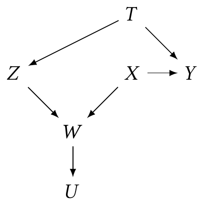
- What must you condition on to estimate the causal effect of \(X\) on \(Y\)?
- If we have selected on \(W = w\), what variables must we condition on, if any, to estimate the causal effect of \(X\) on \(Y\)?
Exercise 2.7 (Conditions for Simpson’s paradox) Simpson’s paradox, as illustrated in Example 2.14, is integrally connected with confounding. If \(X\) is the treatment, \(Y\) is the outcome, and \(Z\) is a confounding variable, and all three are binary, the paradox is that it is possible for the following to be true simultaneously (or their reverse): \[\begin{align*} \Pr(Y=1 \mid Z=1, X=1) &> \Pr(Y=1 \mid Z=1, X=0) & (1)\\ \Pr(Y=1 \mid Z=0, X=1) &> \Pr(Y=1 \mid Z=0, X=0) & (2)\\ \Pr(Y=1 \mid X=1) &< \Pr(Y=1 \mid X=0). & (3) \end{align*}\] Show that this paradox cannot occur if \(X\) and \(Z\) are independent by using the law of total probability. Comment on the connection between this probabilistic result and the causal diagrams: the paradox cannot occur if what is true about the diagram connecting \(X\), \(Y\), and \(Z\)?
Exercise 2.8 (COVID testing) During the COVID pandemic, regular testing was recommended as a strategy to limit spread. Many people sought COVID tests before traveling or visiting vulnerable relatives, after large events, or when they felt sick; some employers required employees to get regularly tested; and some state and federal agencies mandated regular testing among specific groups, such as healthcare workers. But access to testing was uneven: the supply was sometimes limited, it was often difficult to figure out how to get tests, and though tests were supposed to be free or covered by insurance, the expense and paperwork may have deterred some people. Other people chose not to test because they felt their personal risk was low, they felt the pandemic was overblown, or they otherwise didn’t think tests were necessary.
A government agency is interested in creating workplace programs to encourage people to get tested. Suppose they want to know in which occupations people are more or less likely to get a COVID test, and how much of this effect is due to the occupation—due to the job itself, not just because the job involves workers of different demographic groups in different states with different policies.
For example, if healthcare workers get more COVID tests than construction workers, the government agency wants to know if that’s because of their job (and work requirements) or if it’s because healthcare workers have, on average, more education and higher incomes.
- Draw a causal diagram of factors relevant to COVID testing and the agency’s research question. This is open-ended: use your knowledge to think of relevant factors, including ones not listed here, and how they fit into the diagram.
- Based on your diagram, what kind of data should the agency collect to answer their research question? What factors must be included in the data?
Exercise 2.9 (Flight delays) The Bureau of Transportation Statistics collects data on every commercial airline flight in the United States, including the length of any flight delays and their causes. Suppose you have access to the following variables for thousands of flights:
- Departure delay. How late the airplane was when it left the gate to take off
- Arrival delay. How late the airplane was when it arrived at the destination
- Time of flight. How long the airplane spent in the air
- Distance. The distance between the origin and destination of the flight
You have an idea. When an airplane departs late, but it’s a long-distance flight, the pilot might be able to make up for lost time: by going a little bit faster they may be able to catch up and arrive on time. But if it’s a short-distance flight, going a bit faster will only save a minute or two, and won’t have a substantial effect on the arrival delay. So: if two planes both depart late by the same amount, is the one with the longer distance to fly more likely to arrive on time?
- Draw a causal diagram for this situation, including the variables listed above. It may also make sense to add additional variables not shown above, if you think they’re relevant, such as potential confounding variables or variables that influence the relationships between those shown above.
- Which causal relationship would we need to estimate to test your idea? Which variables must be conditioned on to do so? Point to specific paths in the diagram you want to estimate.
- What regression model should you fit to estimate that relationship? Assume the relationships are all linear, and write out a model like \(\text{outcome} = \beta_0 + \beta_1 \text{variable}\)…
- If you fit a regression model to predict arrival delay with all the covariates listed above, does this satisfy the backdoor criterion for the causal effect of interest? What would the interpretation of the distance coefficient be?
Exercise 2.10 (Petting zoo) Recently, Cranberry Melon University installed an on-campus petting zoo to help students relax. A psychology professor is interested in whether spending time with the ducks at the petting zoo causes students to get better grades.
The professor conducts a survey5 of students and records the following variables:
Grade point average. This is the main outcome variable: the student’s GPA a semester after the ducks appeared.
Duck time. Time, during that semester, the student spent with the ducks.
Aptitude. The student’s SAT score from when they were admitted to Cranberry Melon. The psychologist was worried that SAT scores (and aptitude generally) may affect GPA as well as time spent with the ducks.
Dean’s List. Did the student appear on the Dean’s List? Students are put on the Dean’s List based on their GPA and sometimes their extraordinary SAT scores.
Socio-economic status. Measured by family income. This may affect aptitude and GPA, and could be confounded with duck time as well.
Salary after graduation. Affected by many factors—but employers definitely do not know how much time students spend with ducks, because of federal anti-duck-discrimination law.
- Draw a plausible causal diagram incorporating these variables.
- Identify the specific causal path the professor wants to estimate by giving the start and end nodes and all nodes on the path (e.g. \(A \to B \to \cdots \to Z\)).
- Name a minimum set of variables the professor must include in a model to be able to estimate that causal path. Specify the outcome variable and the variables that must be controlled for. Remember, this is an observational survey, not an experiment; but assume all students are equally likely to respond to the survey.
- Identify any variables that the psychologist must not include in the model, if any. Explain (in a sentence or two) why they must not be included.
Exercise 2.11 (SAT scores, Ramsey and Schafer (2013), section 12.1.1) Since 1926, many prospective American college students have taken the SAT before applying to college. In 1982, average scores by state were published by the College Entrance Examination Board (now the College Board), developers of the test. These averages showed large differences by state, from an average score of 790 out of 1600 in South Carolina to an average of 1088 in Iowa. Naturally many people were interested in the source of the differences.
Researchers compiled several possible factors associated with each state’s average score:
- Takers: The percentage of eligible high school seniors in the state who took the SAT. Not every college required the SAT for admission; in some midwestern states, most colleges used other tests, so the only students taking the SAT were those applying to other colleges out of state.
- Income: The median income of families of the students who took the SAT.
- Years: The average number of school years that the students taking the SAT had of courses in social science, humanities, and the natural science.
- Public: The percentage of the SAT takers who attended public high schools, rather than private schools.
- Expend: The total state expenditure on high schools, in hundreds of dollars per student.
- Rank: The median percentile ranking of the test-takers among their high school classes.
Later, we will try to use this data to answer a simple question: Which states have the best performance relative to the amount of money they spend? That is, which get the highest scores per dollar, after accounting for other factors that may influence the scores?
To approach this problem, we should first try to understand the relationships of the variables. Draw a plausible causal diagram of how these factors are related to each other, keeping in mind that the data gives averages per state, and is not at the individual student level. Write a paragraph justifying your choices of arrows and explaining what causal effects you expect.
An earlier version of this joke is due to Wasserman (1999) (“There are two types of statisticians: those who do causal inference and those who lie about it.”). This is only partly a joke: You will find many research papers that are careful not to claim any causal relationship, only an “association”, but that are accompanied by editorials and press releases that assume the association is causal. These researchers are, in other words, attempting to make causal claims while avoiding the obvious criticism that their data and methods cannot justify causal claims.↩︎
A notable exception is the crossover trial, where participants receive one treatment, then “cross over” to the other group and receive the other treatment.↩︎
However, there are equivalence classes of causal diagrams that have different edges but imply the same independence structure. We can’t distinguish between elements of these equivalence classes using data alone.↩︎
Percutaneous nephrolithotomy is an extremely intimidating name, but in Latin it makes perfect sense: per- (through) cutaneous (skin) nephro- (kidney) lith- (stone) otomy (removal).↩︎
The survey is, of course, named the Quantitative Undertaking for Anatidae Cuddling Knowledge.↩︎