5 Geometric Multiple Regression

Consider the linear regression model \(\E[Y \mid X] = r(X) = \beta\T X\), where \(Y \in \R\), \(X \in \R^p\), and \(\beta \in \R^p\). We do not know the true relationship, so we need to obtain a sample from the population and estimate it.

5.1 Regression in the population

Before we fit regression models to samples, we should consider: What is the ideal linear relationship in the population? We assume \(X\) and \(Y\) are drawn jointly from some population distribution, and we want to find the best line relating them.

To define “best”, we have many options, but suppose we choose squared error. Then we can say that the best linear relationship in the population is \(Y = \beta\T X\), where \[ \beta = \argmin_\beta \E[(Y - \beta\T X)^2]. \] We can find \(\beta\) by differentiating and finding the minimum: \[\begin{align*} \frac{\partial}{\partial \beta} \E[(Y - \beta\T X)^2] &= 2 \E[(Y - \beta\T X) X] \\ 0 &= 2 \E[YX] - 2 \E[(\beta\T X) X]\\ \beta\T \E[XX\T] &= \E[YX]\\ \beta &= \E[XX\T]^{-1} \E[YX]. \end{align*}\] This defines the best linear approximation of \(Y\) using \(X\).

Notice we did not need any assumptions to define this quantity. We did not assume that the true form of \(\E[Y \mid X\) is linear or that \(X\) or \(Y\) have any specific distributions. Perhaps the true relationship is nonlinear; nonetheless, there is a best linear approximation. The objective of linear regression will be to find this approximation, and eventually to expand \(X\) so that it is a better approximation.

5.2 Least-squares estimation

Now we consider how to estimate the model using only a sample of \(n\) observations of \(X\) and \(Y\) from the population. Given these observations, we can form the matrix version of this model: \[\begin{align*} \Y &= \begin{pmatrix} y_1 \\ y_2 \\ \vdots \\ y_n \end{pmatrix} & \X &= \begin{pmatrix} x_{11} & \cdots & x_{1p} \\ x_{21} & \cdots & x_{2p} \\ \vdots & \vdots & \vdots \\ x_{n1} & \cdots & x_{np} \end{pmatrix} \end{align*}\]

Our model is now \(\E[\Y \mid \X] = r(X) = \X \beta\). In other words, the model claims that \(\E[\Y \mid \X] \in C(\X)\), the column space of \(\X\).

Often the first column of \(\X\) is a column of ones, to give the model an intercept that is not fixed at 0. We can add other types of columns to \(\X\) to expand the model or make it more flexible, as we will discuss in Chapter 7 and Chapter 10. The columns of \(\X\) are called regressors.

To estimate the unknown parameter vector \(\beta\), we need some criterion for choosing the estimate \(\hat \beta\) that “best” fits the data, i.e. we need some definition of “best”. A reasonable criterion is to choose the \(\hat \beta\) so that the observed \(\Y\) is as close as possible (in Euclidean distance) to the column space of the observed \(\X\). In other words, we choose \(\hat \beta\) by solving \[\begin{align*} \hat \beta &= \argmin_\beta (\Y - \X \beta)\T (\Y - \X \beta) \\ &= \argmin_\beta \|\Y - \X \beta\|_2^2\\ &= \argmin_\beta \RSS(\beta), \end{align*}\] where \(\RSS\) stands for “residual sum of squares” and the norm \(\|\cdot\|_2\) is defined as in Definition 3.7. This criterion chooses the \(\hat \beta\) that minimizes the Euclidean distance between \(\Y\) and \(\X \hat \beta\).

5.2.1 Estimating the slopes

To find the optimal \(\hat \beta\), you may have previously seen derivations that take the derivative of \(\RSS(\beta)\) with respect to \(\beta\), set it to zero, and use this to find the minimum. Instead, let’s consider a geometric result.

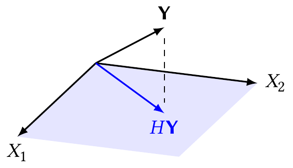
Theorem 5.1 (Least squares estimator) A particular \(\hat \beta\) is the least squares estimate if and only if \(\X \hat \beta = H \Y\), where \(H\) is the perpendicular projection operator onto \(C(\X)\).

Proof. We will show that \[ \RSS(\beta) = \underbrace{(\Y - H \Y)\T (\Y - H \Y)}_{(1)} + \underbrace{(H \Y - \X \beta)\T (H \Y - \X \beta)}_{(2)}, \] where term (1) does not depend on \(\beta\). To minimize the left-hand side with respect to \(\beta\), we need only minimize term (2) with respect to \(\beta\). Term (2) is nonnegative (because it is a norm) and is 0 if and only if \(\X \beta = H \Y\).

To show this, we expand the definition of RSS by adding and subtracting \(H\Y\): \[ \RSS(\beta) = (\Y - H\Y + H\Y - \X \beta)\T(\Y - H\Y + H\Y - \X \beta). \] Multiplying this out yields four terms: \[\begin{align*} \RSS(\beta) ={}& (\Y - H \Y)\T (\Y - H \Y)\\ & + (\Y - H \Y)\T (H \Y - \X \beta)\\ & + (H \Y - \X \beta)\T (\Y - H \Y)\\ & + (H \Y - \X \beta)\T (H \Y - \X \beta), \end{align*}\] but fortunately the second and third terms are zero, because \[ (\Y - H \Y)\T (H \Y - \X \beta) = \Y\T (I - H)H \Y - \Y\T (I - H) \X \beta, \] if we expand and regroup terms. Here \(I\) represents the identity matrix, and \((I - H)H\) and \((I - H)\X\) are both zero because \((I - H)\) is the projection onto the orthogonal complement of the column space of \(\X\) (Theorem 3.4). We are left with only the first and last terms, which is the desired result.

Figure 5.1: Least squares as projection. Let \(n = 3\), and let \(X_1\) and \(X_2\) represent the first and second columns of \(\X\). They span a subspace of \(\R^3\), shown in blue. The response \(\Y\) is another point in \(\R^3\), and the fit \(H\Y\) is the perpendicular projection onto that subspace.

This gives us a useful geometric interpretation of multiple regression, shown in Figure 5.1. The regressors—the columns of \(\X\)—span a subspace of \(\R^n\). The observed \(\Y\) lies some distance from that subspace. We choose the \(\hat \beta\) so that the subspace and \(\Y\) are as close together as possible, in Euclidean distance.

This does not, however, tell us what \(H\) is. But we can work it out. Because it is the projection onto \(C(\X)\), we know \(\X\T(\Y - H \Y) = 0\), because \(\Y - H \Y\) is a vector orthogonal to the column space. Hence \[\begin{align*} \X\T (\Y - H \Y) &= 0\\ \X\T\Y &= \X\T H \Y\\ \X\T\Y &= \X\T \X \hat \beta \\ \hat \beta &= (\X\T\X)^{-1} \X\T \Y, \end{align*}\] applying Theorem 5.1. And since \(\X \hat \beta = H \Y\), \[ \X \hat \beta = \underbrace{\X (\X\T\X)^{-1} \X\T}_{H} \Y, \] and we have a closed form for \(H\), matching Definition 3.16. Similarly, we can write our estimator as \[ \hat \beta = (\X\T \X)^{-1} \X\T \Y. \]

5.2.2 Estimating the error variance

Let us suppose the model is true and \(\E[\Y \mid \X] = \X \beta\). Let us also define \(e = \Y - \X \beta\), so \(e\) is a vector of errors. By definition, \(\E[e \mid \X] = 0\). We can think of these errors as representing measurement error, noise, or unmeasured factors that are associated with the outcome.

The variance of these errors will be important below, in Theorem 5.3, for calculating the sampling distribution of \(\hat \beta\). Unfortunately we usually have no way to know the variance of the errors a priori, so we must estimate the variance after fitting the model.

Theorem 5.2 (Unbiased estimation of error variance) If \(\E[\Y \mid \X] = \X \beta\), where \(\X\) has rank \(p\), and if \(\var(e) = \sigma^2 I\), then \[ S^2 = \frac{(\Y - \X \hat \beta)\T (\Y - \X \hat \beta)}{n - p} = \frac{\RSS(\hat \beta)}{n - p} \] is an unbiased estimate of \(\sigma^2\).

Proof. We have that \[ \Y - \X \hat \beta = (I - H) \Y, \] based on the results of the previous section. Rearranging the estimator and substituting this in, we have \[\begin{align*} (n - p) S^2 &= \Y\T(I - H)\T (I - H) \Y\\ &= \Y\T (I - H)^2 \Y\\ &= \Y\T (I - H) \Y, \end{align*}\] because projection matrices are symmetric and idempotent (Theorem 3.3). To complete the proof, we require an additional result (Seber and Lee 2003 theorem 1.5): if \(A\) is a symmetric matrix and \(b\) is a vector of random variables, where \(\E[b] = \mu\) and \(\var(b) = \Sigma\), then \[ \E[b\T A b] = \trace(A \Sigma) + \mu\T A \mu. \] Applying that here, \[\begin{align*} \E[\Y\T (I - H) \Y] &= \sigma^2 \trace(I - H) + \E[\Y]\T (I - H) \E[\Y] \\ &= \sigma^2 (n - r) + \beta\T \X\T (I - H) \X \beta \\ &= \sigma^2 (n - r), \end{align*}\] because \(H \X = \X\). Hence \(\E[S^2] = \sigma^2\).

TODO Show \(S^2 \sim \chi^2\), as prelude for F tests and such

5.3 Properties of the estimator

Why should we use the least-squares estimator over any other way to estimate \(\hat \beta\)? So far we have given no statistical justification, only the intuition that the least squares criterion chooses \(\hat \beta\) to make \(\Y\) “close to” \(\X \hat \beta\).

Let’s add some statistical justification.

Theorem 5.3 (Properties of the least squares estimate) When \(\E[\Y \mid \X] = \X \beta\) and we use least squares to estimate \(\hat \beta\),

The estimate is unbiased: \(\E[\hat \beta \mid \X] = \beta\).
The sampling variance of the estimator is \[ \var(\hat \beta \mid \X) = (\X\T\X)^{-1} \X\T \var(\Y \mid \X) \X (\X\T \X)^{-1}, \] and if we are willing to assume that \(\var(e \mid \X) = \sigma^2 I\), i.e. the errors are independent and have equal variance, then the sampling variance reduces to \[ \var(\hat \beta \mid \X) = \sigma^2 (\X\T\X)^{-1}. \]
If we are also willing to assume the errors \(e\) are normally distributed, \[ \hat \beta \sim \normal(\beta, \sigma^2 (\X\T \X)^{-1}). \]
If we are not willing to assume the errors are normally distributed, but they have finite variance, then as \(n \to \infty\), \[ \hat \beta \convd \normal(\beta, \sigma^2 (\X\T\X)^{-1}). \]

Proof.

Unbiasedness: \[\begin{align*} \E[\hat \beta \mid \X] &= \E[(\X\T \X)^{-1} \X\T \Y \mid \X] \\ &= (\X\T \X)^{-1} \X\T \E[\Y \mid \X] \\ &= (\X\T \X)^{-1} \X\T \X \beta \\ &= \beta. \end{align*}\]
Sampling variance: \[\begin{align*} \var(\hat \beta \mid \X) &= \var((\X\T\X)^{-1} \X\T \Y \mid \X) \\ &= (\X\T\X)^{-1} \X\T \var(\Y \mid \X) \X (\X\T \X)^{-1}. \end{align*}\] To simplify this, note that \[\var(\Y \mid \X) = \var(\Y - \X \beta \mid \X) = \var(e \mid \X).\] When \(\var(e \mid \X) = \sigma^2 I\), pull \(\sigma^2\) out and cancel \(\X\T\X\) and its inverse, yielding \(\sigma^2 (\X\T\X)^{-1}\).
Normality: Expand the estimator to \(\hat \beta = (\X\T\X)^{-1} \X\T (\X\beta + e)\). The only random variable is \(e\), which is assumed to be normally distributed with mean \(\zerovec\) and variance \(\sigma^2 I\).

A property of normal distributions is that shifting or scaling them by constants yields another normal distribution. We obtained the mean and variance in parts 1 and 2 of this proof.
Asymptotic normality: Because \(\hat \beta\) is a linear combination of random variables (\(\Y\)) with fixed weights (\((\X\T\X)^{-1} \X\T\)), we can apply the Lindeberg–Feller central limit theorem.

Notice that these results are conditional on \(\X\): we showed that the conditional expectation of \(\hat \beta\) is \(\beta\). Typically, theoretical results for regression are conditioned on \(\X\), or equivalently treat \(\X\) as fixed. The only source of randomness (in expectations, variances, and so on) is the error \(e\), which we assume to have mean 0.

If \(\X\) is sampled from a population and considered to be random, it is straightforward to extend these results: a result that holds when conditioned on any \(\X\) will hold in general for \(\X\) sampled from the population. But if \(\X\) is observed with random error, we will encounter problems. We will explore this later.

Next, we can use these basic results to show that the least squares estimate has other useful properties. It is nice for estimators to be unbiased, and it is also nice for them to have minimal variance, so \(\hat \beta\) tends to be close to \(\beta\). We can define this formally.

Definition 5.1 (Minimum variance linear unbiased estimator) An estimator is linear if it is a linear combination of the entries of \(\Y\), e.g. \(a\T \Y\), for \(a \in \R^n\) that may depend on \(\X\).

An estimator \(a\T \Y\) is the minimum variance linear unbiased estimator if it is unbiased and if for any other linear unbiased estimate \(b\T \Y\), \(\var(a\T \Y) \leq \var(b\T \Y)\).

Suppose we would like to estimate a target quantity \(a\T \X \beta\), where \(a \in \R^n\). For instance, if we choose \(a\T = (\X\T \X)^{-1} \X\T\), our target quantity is \(\beta\); but we can choose \(a\) to estimate other quantities as well.

Theorem 5.4 (Gauss–Markov theorem) Consider a regression model where \(\E[\Y \mid \X] = \X \beta\), where the errors \(e\) are uncorrelated and have common variance \(\sigma^2\). To estimate a quantity \(a\T \X \beta\), the estimator \(a\T \X \hat \beta\), where \(\hat \beta\) is the least squares estimator defined above, is the unique minimum variance linear unbiased estimate (Seber and Lee 2003, Theorem 3.2).

Proof. Let \(b\T \Y\) be any other linear unbiased estimate of \(a\T \X \beta\). Then \[ a\T \X \beta = \E[b\T \Y] = b\T \E[Y] = b\T \X \beta, \] so \((a - b)\T \X \beta = 0\). This implies the vector \(a - b\) is orthogonal to the column space of \(\X\), and hence \(H(a - b) = 0\) and \(Ha = Hb\).

We can now consider the variance of the estimator: \[\begin{align*} \var(a\T \X \hat \beta) &= \var((Ha)\T \Y) \\ &= \var((Hb)\T \Y) \\ &= \sigma^2 b\T H\T H b \\ &= \sigma^2 b\T H^2 b \\ &= \sigma^2 b\T H b, \end{align*}\] because \(H\) is idempotent. Hence the difference in variance of the estimators is \[\begin{align*} \var(b\T \Y) - \var(a\T \X \hat \beta) &= \var(b\T \Y) - \var((Hb)\T Y) \\ &= \sigma^2 (b\T b - b\T H b) \\ &= \sigma^2 b\T (I - H) b \\ &= \sigma^2 \underbrace{b\T (I - H)\T}_{d_1\T} \underbrace{(I - H) b}_{d_1} \\ &= \sigma^2 d_1\T d_1 \\ &\geq 0, \end{align*}\] with equality if and only if \((I - H) b = 0\), which would imply \(b = H b = H a\), and hence \(a = b\).

So any other linear unbiased estimate has greater variance unless it is identical.

Notice this result does not depend on the exact distribution of the errors, only that they are uncorrelated with a common (and finite) variance. The errors need not be normally distributed for this useful property to hold.

Of course, we need not use a linear unbiased estimate of \(\beta\); we could choose to use a nonlinear biased estimate if we had good reason. We will see later that there can be good reasons, particularly when there are many regressors relative to the amount of the data, or when we are more interested in minimizing prediction error than in estimating \(\beta\) perfectly.

5.4 Inference

5.4.1 Parameters

Theorem 5.3 tells us that, when the errors are normally distributed with common variance, \(\hat \beta \sim \normal(\beta, \sigma^2 (\X\T\X)^{-1})\). We of course observe \(\X\), but \(\sigma^2\) is an unknown parameter, so we must use Theorem 5.2 to estimate it. This leads to the following result.

Theorem 5.5 (t statistic for regression estimates) When \(\hat \beta\) is estimated using least squares, and when the conditions in Theorem 5.3 hold, our estimate of the marginal variance of \(\hat \beta_i\) is \[ \widehat{\var}(\hat \beta_i) = S^2 (\X\T\X)^{-1}_{ii}, \] using the estimate \(S^2\) from Theorem 5.2, and where \(A_{ii}\) represents the entry in the \(i\)th row and column for a matrix \(A\). Consequently, \[ \frac{\hat \beta_i - \beta_i}{\sqrt{\widehat{\var}(\hat \beta_i)}} \sim t_{n - p}, \] where \(t_{n - p}\) is the Student’s \(t\) distribution with \(n - p\) degrees of freedom. The quantity \[ \se(\hat \beta_i) = S \sqrt{(\X\T\X)^{-1}_{ii}} \] is known as the standard error of \(\hat \beta_i\).

More generally, for any fixed \(a \in \R^p\), \[ \var(a\T \hat \beta) = a\T \var(\hat \beta) a = \sigma^2 a\T (\X\T \X)^{-1} a, \] and so \[ \frac{a\T \hat \beta - a\T \beta}{S \sqrt{a\T (\X\T \X)^{-1} a}} \sim t_{n - p}. \]

(TODO Comments on how this follows because N/chi = t, independence of S2 and beta, etc; maybe follow Christensen?)

We can use this result to derive confidence intervals for individual parameters. Letting \(t_n^\alpha\) denote the \(\alpha\) quantile of the \(t_n\) distribution, a \(1 - \alpha\) confidence interval for \(\beta_i\) is \[ \left[\hat \beta_i + t_{n - p}^{\alpha/2} \sqrt{\widehat{\var}(\hat \beta_i)}, \hat \beta_i + t_{n - p}^{1 - \alpha/2} \sqrt{\widehat{\var}(\hat \beta_i)}\right]. \]

Similarly, we can conduct hypothesis tests for individual coefficients. Suppose the null hypothesis is \(H_0: \beta_i = c\) for some constant \(c\). Let the test statistic be \[ t = \frac{\hat \beta_i - c}{\sqrt{\var(\hat \beta_i)}}. \] Under the null hypothesis, this test statistic is distributed as \(t_{n-p}\), and so a \(p\)-value can be calculated directly. Tests for the null hypothesis with \(c = 0\) are particularly common, and often printed out automatically by regression software. These tests are often misused: rejecting the null hypothesis (no matter how small the \(p\) value) does not imply the association is strong or that the model’s predictions are highly accurate, while failing to reject the null hypothesis does not prove there is no association or that it is better to remove the regressor from the model. The test merely tells us if we have sufficient evidence to conclude the slope is nonzero, or if zero is a plausible value. In complex applied settings, there often is a true association between almost everything, and so almost any test will be significant if given enough data—and so the test becomes a measure of sample size, not of the practical significance of the findings.

5.4.2 Mean function

We can also use Theorem 5.5 to derive confidence intervals for the mean function \(\E[Y \mid X] = r(X)\) evaluated at a specific point \(X = x_0\). Let \(a = x_0\); then \[ \frac{x_0\T \hat \beta - x_0\T \beta}{S \sqrt{a\T (\X\T \X)^{-1} a}} \sim t_{n - p}, \] allowing us to specify a confidence interval for \(r(x_0)\) as \[ \left[ x_0\T \hat \beta + t_{n-p}^{\alpha/2} S \sqrt{x_0\T (\X\T \X)^{-1} x_0}, x_0\T \hat \beta + t_{n-p}^{1 - \alpha/2} S \sqrt{x_0\T (\X\T \X)^{-1} x_0}\right]. \] This is a pointwise interval, meaning that it has nominal \(1 - \alpha\) coverage when used to make a confidence interval for any particular point \(X = x_0\). However, if we make many such confidence intervals so we can draw a confidence band around the regression line over a range of \(X\) values, this band will have coverage less than \(1 - \alpha\). TODO Scheffe, or maybe put that later in prediction?

5.4.3 Predictions

Confidence intervals for the mean function can easily be misinterpreted. They give uncertainty for our estimate of the mean, but each observation \(Y\) varies around the mean according to the error variance \(\sigma^2\). The result is that a 95% confidence interval for the mean need not include 95% of observations; indeed, usually it contains far fewer than 95% of the observations, since the variance of the mean is smaller than the variance of the individual observations.

If we are truly interested in the mean, that is fine. But sometimes we are interested in making predictions. If we observe \(X = x_0\), what is our prediction for the corresponding \(Y\), and how far will that prediction be from the true \(Y\)? We can form a prediction interval for the individual observation; a 95% prediction interval should contain 95% of observations. The prediction interval adds the variance of the residuals to the variance in the estimate of the mean: \[ \left[ x_0\T \hat \beta + t_{n-p}^{\alpha/2} S \sqrt{1 + x_0\T (\X\T \X)^{-1} x_0}, x_0\T \hat \beta + t_{n-p}^{1 - \alpha/2} S \sqrt{1 + x_0\T (\X\T \X)^{-1} x_0}\right]. \]

5.5 The residuals

So far we have defined the vector of errors as \(e = \Y - \X \beta\). These errors are unknown and unobservable. But we can estimate \(\hat \Y = \X \hat \beta\), and then define the residuals, which are the difference between observed and estimated values of \(\Y\): \(\hat e = \Y - \hat \Y\).

We can write the residuals as \[\begin{align*} \hat e &= \Y - \hat \Y \\ &= \Y - \X \hat \beta \\ &= \Y - \X (\X\T \X)^{-1} \X\T \Y \\ &= (I - H) \Y. \end{align*}\]

5.5.1 Properties of the residuals

Because the residuals are calculated using the observed data and \(\hat \beta\), they are correlated and may have unequal variance even when the true errors are independent with equal variance.

Theorem 5.6 (Variance of the residuals) If \(\var(e \mid \X) = \sigma^2 I\), then \[\begin{align*} \var(\hat e \mid \X) &= \var((I - H) \Y \mid \X) \\ &= (I - H) \sigma^2, \end{align*}\] because \(I - H\) is fixed and idempotent, and \(\var(\Y \mid \X) = \sigma^2 I\). This variance matrix is not diagonal.

Hence the variance of the \(i\)th residual \(\hat e_i\) is \[ \var(\hat e_i) = \sigma^2 (1 - h_{ii}), \] where \(h_{ii}\) is the \(i\)th diagonal entry in \(H\).

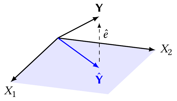
Next, if we think of the geometry of multiple regression as a projection, we can see several interesting results. As shown in Figure 5.2, the least-squares fitted value \(\hat \Y = H \Y\) is the projection of \(\Y\) onto the column space of \(\X\), and therefore the residual vector \(\hat e = \Y - H \Y\) is perpendicular to the columns of \(\X\). It must be perpendicular, because only the perpendicular projection minimizes \(\|\Y - \hat \Y\|_2\).

Figure 5.2: Residuals as projections. As in Figure 5.1, let \(n = 3\), and let \(X_1\) and \(X_2\) represent the first and second columns of \(\X\). The vector from \(\hat \Y\) to \(\Y\) is the residual vector \(\hat e\), forming a right triangle.

To see this algebraically, consider any vector \(a \in \R^p\), so that \(\X a\) is an arbitrary vector in the column space of \(\X\). We have \[\begin{align*} (\Y - H\Y)\T \X a &= \Y\T \X a - \Y\T H\T \X a\\ &= \Y\T \X a - \Y\T \X a\\ &= 0, \end{align*}\] because \(H\T\X = H\X = \X\). Hence the inner product between \(\hat e = \Y - H \Y\) and any vector in the column space of \(\X\) is 0, and the residuals are orthogonal to \(\X\). We should be careful to note, however, that this only applies if \(\hat \beta\) is the least squares estimate—if it is not, \(\hat Y \neq H \Y\), and this result may not hold.

The geometric relationship helps us see key facts. For example: If we expand the column space of \(\X\), we must either get the same \(\RSS(\hat \beta)\) (if the perpendicular projection onto the column space is still the same distance away) or a smaller one; we cannot get a larger \(\RSS(\hat \beta)\) except by reducing or changing the column space of \(\X\). Adding more regressors, or adding transformations of existing regressors, hence can only decrease \(\RSS(\hat \beta)\).

5.5.2 Standardized residuals

As the observed residuals have unequal variance (Theorem 5.6), it can be useful to standardize them so they have equal variance if the model assumptions are correct. In Chapter 9, we will discuss ways to check if the model assumptions hold and we have chosen a reasonable model, and standardized residuals will feature heavily there—because if plots of the standardized residuals show unequal variance or strange trends, we have a strong hint the model does not fit the data well.

Definition 5.2 (Standardized residuals) The standardized residual \(r_i\) for observation \(i\) is \[ r_i = \frac{\hat e_i}{S \sqrt{1 - h_{ii}}}, \] which is the observed residual divided by an estimate of its standard deviation. Here \(S\) is an estimate of \(\sigma\), as given in Theorem 5.2.

When the model assumptions hold, the standardized residuals have mean 0 and variance approximately 1. (The variance is approximate because we use the estimate \(S\), not the true \(\sigma\).) We will use this property in Chapter 9 to construct diagnostics that help us check if the model assumptions hold in particular datasets.

When there are a few observations with very large residuals \(\hat e_i\), the estimated error \(\hat \sigma^2\) will be large, shrinking the standardized residuals. We can make the outlying observations more obvious by using the Studentized residuals.

Definition 5.3 (Studentized residuals) The Studentized residual \(t_i\) for observation \(i\) is \[ t_i = \frac{\hat e_i}{S^{(i)} \sqrt{1 - h_{ii}}}, \] where \(S^{(i)}\) is the residual standard deviation estimated with observation \(i\)’s residual omitted.

Beware of names. The name “Studentized” is sometimes applied to the standardized residuals instead; other textbooks refer to “internally Studentized” (standardized) and “externally Studentized” residuals. Our naming matches R’s, but if you use other books or sources, check what the names refer to.

5.5.3 Partial residuals

Until now, we’ve written the linear regression model in matrix or vector form. Let’s write out the model as a sum instead: \[ Y = \sum_{j=1}^p \beta_j X_j + e. \] Suppose we are not sure if a particular regressor \(X_k\) is linearly related to \(Y\) or related in a more complicated way, such as through an unknown function \(g\): \[ Y = g(X_k) + \sum_{j \neq k} \beta_j X_j + e. \tag{5.1}\] If we fit a linear model and obtain estimates \(\hat \beta\), we can obtain partial residuals, which can help us visualize the possible shape of \(g\).

Definition 5.4 (Partial residuals) The partial residual \(r_{ij}\) for observation \(i\) and regressor \(j\) is \[ r_{ij} = \hat e_i + \hat \beta_j x_{ij}. \]

Why is this useful? The \(i\)th residual \(\hat e_i\) is \[ \hat e_i = y_i - \sum_{k=1}^p \hat \beta_k x_{ik}, \] so we substitute in Equation 5.1 to define \(y_i\), we have \[ \hat e_i = g(x_{ij}) + \sum_{k \neq j} \beta_k x_{ik} + e_i - \sum_{k=1}^p \hat \beta_k x_{ik}. \] Substituting this into the definition of the partial residuals, we obtain \[\begin{align*} r_{ij} &= g(x_{ij}) + \sum_{k \neq j} \beta_k x_{ik} + e_i - \sum_{k=1}^p \hat \beta_k x_{ik} + \hat \beta_j x_{ij} \\ &= g(x_{ij}) + \sum_{k\neq j} \beta_k x_{ik} + e_i - \sum_{k \neq j} \hat \beta_k x_{ik} \\ &= g(x_{ij}) + \sum_{k \neq j} (\beta_k - \hat \beta_k) x_{ik} + e_i. \end{align*}\] If \(\beta_k \approx \hat \beta_k\), then the second term will be small and plotting \(r_{ij}\) against \(x_{ij}\) should reveal the shape of \(g\).

That is, of course, a big “if”. But under reasonable conditions, the partial residual plot will reveal the approximate shape of \(g\), and can help us evaluate if that shape is linear (in which case a linear model is appropriate) or not. See Cook (1993) for details on the conditions and interpretation.

Partial residuals can also be expanded to account for models with interactions and nonlinear terms, as we will see in Section 7.6, making them a versatile way to explore the model’s fitted relationships.

5.6 Exercises

Exercise 5.1 (Variable scaling) Consider a design matrix \(\X\). Suppose it has \(n\) rows and \(p\) columns.

In ordinary least squares regression, we have the model \(\Y = \X \beta\) and estimate \(\hat \beta\).

Suppose we pick some column \(k\) in \(\X\) and divide all its entries by 7. Call this new design matrix \(\X^*\) and the corresponding least squares fit \(\hat \beta^*\)

Will the fitted values \(\hat \Y^* = \X^* \hat \beta^*\) from the model change? Briefly explain why or why not.
What is the relationship between the two coefficients estimates \(\hat \beta_k\) and \(\hat \beta_k^*\) for the covariate \(k\) we rescaled? Give an equation relating the two.
Using the results of Section 5.4.1, we can calculate confidence intervals and \(p\) values for \(\hat \beta_k^*\). How would these differ from the confidence intervals and \(p\) values for \(\hat \beta_k\)? Be specific.

Exercise 5.2 (Sum of the residuals) Consider a linear regression conducted with an intercept, so the design matrix contains a column of ones: \[ \X = \begin{pmatrix} 1 & x_{11} & \cdots \\ 1 & x_{21} & \cdots \\ \vdots & \vdots & \\ 1 & x_{n1} & \cdots \end{pmatrix}. \] Using only the geometric results given above, show that the sum of the residuals is \[ \sum_{i=1}^n \hat e_i = 0. \]