12 Logistic Regression
\[ \DeclareMathOperator{\E}{\mathbb{E}} \DeclareMathOperator{\R}{\mathbb{R}} \DeclareMathOperator{\RSS}{RSS} \DeclareMathOperator{\AIC}{AIC} \DeclareMathOperator{\bias}{bias} \DeclareMathOperator{\MSE}{MSE} \DeclareMathOperator{\VIF}{VIF} \DeclareMathOperator{\var}{Var} \DeclareMathOperator{\cov}{Cov} \DeclareMathOperator{\cor}{Cor} \DeclareMathOperator{\se}{se} \DeclareMathOperator{\trace}{trace} \DeclareMathOperator{\vspan}{span} \DeclareMathOperator{\proj}{proj} \newcommand{\condset}{\mathcal{Z}} \DeclareMathOperator{\cdo}{do} \newcommand{\ind}{\mathbb{I}} \newcommand{\T}{^\mathsf{T}} \newcommand{\X}{\mathbf{X}} \newcommand{\Y}{\mathbf{Y}} \newcommand{\Z}{\mathbf{Z}} \newcommand{\zerovec}{\mathbf{0}} \newcommand{\onevec}{\mathbf{1}} \newcommand{\trainset}{\mathcal{T}} \DeclareMathOperator*{\argmin}{arg\,min} \DeclareMathOperator*{\argmax}{arg\,max} \DeclareMathOperator{\SD}{SD} \newcommand{\dif}{\mathop{\mathrm{d}\!}} \newcommand{\convd}{\xrightarrow{\mathrm{D}}} \DeclareMathOperator{\logit}{logit} \newcommand{\ilogit}{\logit^{-1}} \DeclareMathOperator{\odds}{odds} \DeclareMathOperator{\dev}{Dev} \DeclareMathOperator{\sign}{sign} \DeclareMathOperator{\normal}{Normal} \DeclareMathOperator{\binomial}{Binomial} \DeclareMathOperator{\bernoulli}{Bernoulli} \DeclareMathOperator{\poisson}{Poisson} \DeclareMathOperator{\multinomial}{Multinomial} \DeclareMathOperator{\uniform}{Uniform} \DeclareMathOperator{\edf}{edf} \]
In logistic regression, we model data where \(Y \in \{0, 1\}\), and we want to understand the relationship between \(X\) and \(Y\). There are many possible data types that involve binary outcomes:
- Do patients recover (\(Y = 1\)) or not (\(Y = 0\)) when given a particular treatment, given their prior health status?
- Can we classify an email as spam (\(Y = 1\)) or ham1 (\(Y = 0\)), based on features of the text inside it?
- In a large sample of people, did those with lung cancer (\(Y = 1\)) smoke more tobacco products than those without lung cancer (\(Y = 0\))?
If each observation \(Y\) is independent of the others when we condition on \(X = x\), then \[ Y \sim \bernoulli(f(x)), \] and learning \(f\) tells us about the relationships of interest.
In this model, because \(Y \in \{0, 1\}\), \(\E[Y \mid X = x] = \Pr(Y = 1 \mid X = x)\). If we used least squares to fit a linear model, just like any other linear model, it would estimate \(\Pr(Y = 1 \mid X = x)\) as a linear function of \(x\), and might even do a good job (Gomila 2021).
But a linear model is often unsatisfactory. It could easily predict probabilities greater than 1 or less than 0, which does not make sense; intuitively, the relationship between predictors and the probability of an outcome must be nonlinear, because a linear relationship can always produce predictions greater than 1 or less than 0. We need some kind of transformation that ensures the model always predicts a valid probability.
One possible transformation is to use the odds. The odds of an event are the probability of the event divided by the probability of the event not occurring: \[ \odds(Y = 1 \mid X = x) = \frac{\Pr(Y = 1 \mid X = x)}{1 - \Pr(Y = 1 \mid X = x)}. \] And while \(\Pr(Y = 1 \mid X = x) \in [0, 1]\), the range of odds is broader: \(\odds(Y = 1 \mid X = x) \in [0, \infty)\). This is promising, because it means that \[ \log(\odds(Y = 1 \mid X = x)) \in (-\infty, \infty). \] Will a model of log-odds make sense?
12.1 The basic model
We can write the basic logistic regression model in term of the logit function and its inverse: \[\begin{align*} \logit(p) &= \log\left( \frac{p}{1 - p} \right) \\ &= \log p - \log(1 - p) \\ \ilogit(x) &= \frac{\exp(x)}{1 + \exp(x)} \\ &= \frac{1}{1 + \exp(-x)}. \end{align*}\] The logit function takes a probability and transforms it into a log-odds. Specifically, a model of the log-odds is a model that \[ \logit(\Pr(Y = 1 \mid X = x)) = f(x), \] where we want to learn the function \(f\) using regression. We call the logit function the link function, because it links the probability to our model \(f(x)\). In logistic regression, just like linear regression, we assume the function \(f\) can be written as a linear combination of \(X\) and a parameter \(\beta\).
Definition 12.1 (Logistic regression) When \(Y \in \{0, 1\}\), \(X \in \R^p\), and \(\beta \in \R^p\), logistic regression models the response as \[ \logit(\Pr(Y = 1 \mid X = x)) = \beta\T x, \] or, equivalently, \[\begin{align*} \Pr(Y = 1 \mid X = x) &= \ilogit (\beta\T x)\\ \odds(Y = 1 \mid X = x) &= \exp(\beta\T x) \\ \log(\odds(Y = 1 \mid X = x)) &= \beta\T x. \end{align*}\] We usually consider \(\hat y_i\), the prediction for observation \(i\), to be the predicted probability: \[ \hat y_i = \widehat{\Pr}(Y = 1 \mid X = x_i) = \ilogit(\hat \beta\T x_i). \]
The responses \(Y\) are assumed to be conditionally independent given the covariates \(X\).
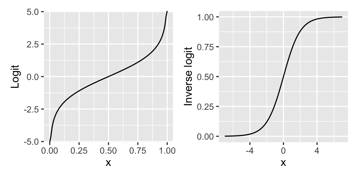
The shape of this relationship is shown in Figure 12.1. When \(x = 0\), \(\ilogit(x) = 1/2\). As \(x\) increases, \(\ilogit(x)\) approaches 1, but never exactly reaches one—hence the S-shaped curve, sometimes known as a “sigmoid” curve.
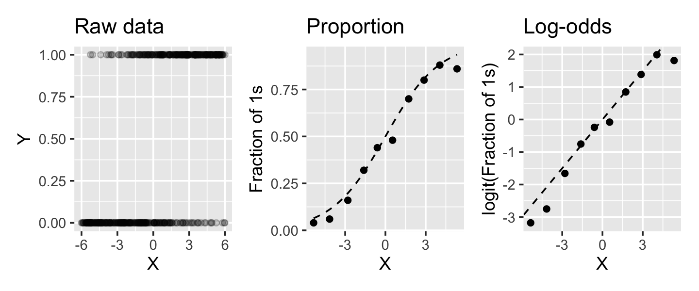
The relationship between the predictor and the predicted proportion and log-odds is shown in Figure 12.2. In the simulated data, \[ \logit(\Pr(Y = 1 \mid X = x)) = \frac{x}{2}. \] The raw data does not show a clear trend because \(Y\) is binary. But if we break the data into chunks and calculate the proportion of observations with \(Y = 1\) in each chunk, we can see the shape of the sigmoid curve, just like in Figure 12.1. If we take the logit of the proportion, we can see it is linearly proportional to \(x\), just as the formula says it should be.
There are a few things to note about this logistic regression model:
- We are modeling (through the logit function) the probability that \(Y = 1\). Our model predicts probabilities (or odds), not actual values of \(Y\). That means we’ll have to adjust how we fit the model, since residuals make less sense here.
- The relationship between \(X\) and the response is nonlinear, so interpreting \(\beta\) will become more challenging.
- None of the geometry from Chapter 5 will help us now! Fitting this model is no longer a projection onto the column space of \(X\), and so many of the useful geometric results that gave us intuition no longer apply here.
12.2 Fitting the model
Because logistic regression gives a specific probability model for \(Y\)—it says \(Y\) is Bernoulli with a particular probability—we can write out the likelihood function directly in terms of an observed dataset \((x_1, y_1), \dots, (x_n, y_n)\): \[ L(\beta) = \prod_{i=1}^n \Pr(y_i = 1 \mid X_i = x_i)^{y_i} \Pr(y_i = 0 \mid X_i = x_i)^{1 - y_i}. \] Because \(y_i \in \{0, 1\}\) and \(a^0 = 1\) for any \(a\), this is just a clever way of writing that each term is \(\Pr(y_i = 1 \mid X_i = x_i)\) when \(y_i = 1\), or \(\Pr(y_i = 0 \mid X_i = x_i)\) when \(y_i = 0\). You can also see this as the binomial probability mass function for a binomial distribution with one trial.
By substituting in the model, taking logs, and simplifying, we can show that the log-likelihood function is \[\begin{align*} \ell(\beta) &= \sum_{i=1}^n y_i \log(\Pr(y_i = 1 \mid X_i = x_i)) + (1 - y_i) \log(\Pr(y_i = 0 \mid X_i = x_i)) \\ &= \sum_{i=1}^n y_i \beta\T x_i - \log\left(1 + e^{\beta\T x_i}\right). \end{align*}\] To estimate \(\hat \beta\), we can proceed by maximum likelihood, by choosing \[ \hat \beta = \argmax_\beta \ell(\beta). \]
Unfortunately, if we try to solve this optimization problem by setting the derivative of \(\ell(\beta)\) equal to zero, we obtain an expression that can’t be analytically solved for \(\beta\).
Instead, statistical software (like R, SAS, scikit-learn, and any other package you are likely to use) maximizes the likelihood using numerical optimization methods. In principle, any numerical optimization method will work: gradient ascent, Newton’s method, or any of a dozen other optimization algorithms you might learn in a numerical methods class (or in Boyd and Vandenberghe 2004). In practice, the details of the optimization algorithm are not important for us as statisticians: the logistic regression likelihood is well-behaved and fairly easy to optimize, so any reasonable method will yield a good solution, and we don’t care what method is used as long as \(\hat \beta\) is very close to the true maximizer. Nonetheless, we’ll mention one commonly used algorithm just because its use is widespread and its details justify some of the other tools we will use for logistic regression.
12.2.1 Iteratively reweighted least squares
You may be familiar with gradient descent because of its popularity in fitting deep neural networks. The same process to maximize, rather than minimize, a function is known as gradient ascent, and the process is straightforward. We start with a guess \(x^{(0)}\). Then, at each iteration \(k\), we:
- Calculate the gradient \(f'(x^{(k)})\). This tells us which direction the function is increasing in.
- Update \(x^{(k + 1)} = x^{(k)} + \eta f'(x^{(k)})\). This moves us “uphill”, in a direction the function is increasing. We must choose the step size \(\eta\), which determines how far we move.
- Repeat until convergence.
Gradient ascent requires us to choose a tuning parameter \(\eta\). If the step size is too large, we may move past the maximum to the other side; if it is too small, it will take many iterations to reach the maximum. But if we know the curvature of \(f(x)\)—that is, if we know its second derivative—we can determine how far to move at each step based on the curvature. If there is strong curvature, take a small step to avoid going past a maximum; if there is almost no curvature, we can safely take a larger step.
This leads us to Newton’s method for optimization. In our case, the log-likelihood is a function \(f : \R^p \to R\), and so we will need to write Newton’s method in terms of the gradient \(Df\) and Hessian \(D^2 f\).
Definition 12.2 (Newton’s method for optimization) Assume there is a point \(x^*\) such that \(D f(x^*) = 0\). If \(f\) is suitably well-behaved, then the iterative update procedure \[ x^{(k + 1)} = x^{(k)} - \left(D^2 f(x^{(k)})\right)^{-1} Df(x^{(k)})\T \] converges quadratically to \(x^*\) whenever \(x^{(0)}\) is sufficiently close to \(x^*\).
Proof. See Humpherys and Jarvis (2020), theorem 12.4.1, and Humpherys et al. (2017), theorem 7.3.12. The basic idea is to approximate \(f(x)\) using second-order Taylor expansion around \(x^{(k)}\). This produces a parabola that locally approximates \(f(x)\). We choose \(x^{(k + 1)}\) to be the maximum of the parabola. When \(f(x)\) is approximately quadratic in shape, the Taylor expansion is a good approximation and this rapidly brings us to the maximum; even when it is not approximately quadratic, the process works fairly well.
Quadratic convergence is fast, i.e., we need fairly few iterations to arrive at a good answer, provided we can choose a good starting point \(x^{(0)}\) and can easily calculate the gradient and Hessian. As we’ll see, it turns out we can meet both of these requirements fairly easily in logistic regression.
Let’s write out these derivatives. We have that \[ D \ell(\beta) = \sum_{i=1}^n x_i \left(y_i - \frac{1}{1 + e^{\beta\T x_i}} \right). \] We can simplify this by defining a vector \(P \in [0, 1]^n\), where \[ P_i = \Pr(Y_i = 1 \mid X_i = x_i) = \frac{1}{1 + \exp(-\beta\T x_i)}. \] We can then write that \[ D \ell(\beta) = \X\T(\Y - P). \]
Next, we can calculate the Hessian as \[\begin{align*} D^2 \ell(\beta) &= - \sum_{i=1}^n x_i x_i\T \left(\frac{1}{1 + \exp(-\beta\T x_i)}\right) \left(1 - \frac{1}{1 + \exp(-\beta\T x_i)}\right) \\ &= -\X\T W \X, \end{align*}\] where \(W\) is an \(n \times n\) diagonal matrix whose diagonal entries are \[ W_{ii} = \left(\frac{1}{1 + \exp(-\beta\T x_i)}\right) \left(1 - \frac{1}{1 + \exp(-\beta\T x_i)}\right) = P_i (1 - P_i). \]
According to Definition 12.2, the iterative optimization procedure is hence \[\begin{align*} \hat \beta^{(n + 1)} &= \hat \beta^{(n)} + (\X\T W \X)^{-1} \X\T (\Y - P) \\ &= (\X\T W \X)^{-1} \X\T W\left(\X \hat \beta^{(n)} + W^{-1} (\Y - P)\right) \\ &= (\X\T W \X)^{-1} \X\T W Z^{(n)}, \end{align*}\] where \(Z^{(n)} = \X \hat \beta^{(n)} + W^{-1}(\Y - P)\). This is the solution to a weighted least squares problem where we are trying to predict \(Z^{(n)}\) from \(\X\) with weights given by \(W\).
Consequently, a logistic regression model can be fit as a sequence of weighted linear regressions, hence the name “iteratively reweighted least squares”, or IRLS. If we replace \(D^2 \ell(\beta)\) with its expectation, we get the related “Fisher scoring” procedure. (Here \(D^2 \ell(\beta)\) is not random, so Fisher scoring and IRLS are identical.) Because of the quadratic convergence of Newton’s method, optimization can take only a few iterations. This method is also appealing because statistical software packages usually already have code to do least squares efficiently, so that code can be reused to implement logistic regression.
However, this is certainly not the only way to obtain the maximum likelihood estimator \(\hat \beta\) for a logistic regression model. Any numerical optimization procedure could work, and while IRLS has advantages, sometimes a different optimizer can be more suitable. For example, for very large datasets the Hessian \(D^2 \ell(\beta)\) is a very large matrix, and the matrix operations required can be quite slow, so every iteration is costly; a procedure like gradient descent or stochastic gradient descent may be easier to run, even if it does require more iterations to converge.
12.2.2 Fitting in R
In R, the glm() function (for “generalized linear model”) can fit logistic regression models. This function also fits other generalized linear models, as we will see in Chapter 13, so we must tell it that our outcome variable has a Binomial distribution (as the Bernoulli is Binomial with one trial). It otherwise works just like lm().
In the model formula, the response variable (on the left-hand side of the ~) can be a binary integer or a factor variable. If it is a factor variable, R will treat the first level of the factor as the baseline and model the probability of the second level, so the predictions will be for the probability of the second level. You can reorder the levels if this causes the predictions to be the opposite of what you want; the fct_relevel() function from the forcats package can be a convenient way to do this.
Example 12.1 (Fitting a basic logistic regression) Let’s use the regressinator to define a population with a binary outcome. We can do this by specifying the family argument of the response() function:
library(regressinator)

logit_pop <- population(
  x1 = predictor(rnorm, mean = 0, sd = 10),
  x2 = predictor(runif, min = 0, max = 10),
  y = response(0.7 + 0.2 * x1 - 0.2 * x2,
               family = binomial(link = "logit"))
)
This definition specifies that \[\begin{align*} Y &\sim \text{Bernoulli}\left(\ilogit(\beta\T X)\right) \\ \beta &= (0.7, 0.2, -0.2)\T, \end{align*}\] where \(X = (1, X_1, X_2)\T\). If we obtain a sample from the population, we can fit the model:
logit_data <- logit_pop |>
  sample_x(n = 500) |>
  sample_y()

fit <- glm(y ~ x1 + x2, data = logit_data, family = binomial())
summary(fit)
Call:
glm(formula = y ~ x1 + x2, family = binomial(), data = logit_data)

Coefficients:
            Estimate Std. Error z value Pr(>|z|)
(Intercept)  0.45107    0.22525   2.003   0.0452 *
x1           0.18471    0.01697  10.887  < 2e-16 ***
x2          -0.16382    0.04094  -4.001  6.3e-05 ***
---
Signif. codes:  0 '***' 0.001 '**' 0.01 '*' 0.05 '.' 0.1 ' ' 1

(Dispersion parameter for binomial family taken to be 1)

    Null deviance: 688.53  on 499  degrees of freedom
Residual deviance: 460.59  on 497  degrees of freedom
AIC: 466.59

Number of Fisher Scoring iterations: 5
This fit required only 5 iterations to converge, according to the output. We will begin to interpret the rest of the output in Section 12.3, but we can at least see that the estimated coefficients are not too far off from the true coefficients.
12.2.3 The shape of the regression function
As we saw in Figure 12.1, the inverse logistic function is nonlinear. We can still think of \(\X \beta\) as defining a plane, of course, but the relationship between \(X\) and \(\Pr(Y = 1 \mid X = x)\) is not linear.
Example 12.2 (The contours of probability) Using the fit from Example 12.1, let’s plot \(\Pr(Y = 1 \mid X_1 = x_1, X_2 = x_2)\) in 3D:
x1s <- seq(-10, 10, by = 1)
x2s <- seq(0, 10, by = 0.5)

z <- outer(x1s, x2s, FUN = function(x1, x2) {
  predict(fit, newdata = data.frame(x1 = x1, x2 = x2),
          type = "response")
})

persp(x1s, x2s, z, theta = 320, xaxs = "i",
      xlab = "X1", ylab = "X2", zlab = "Prob")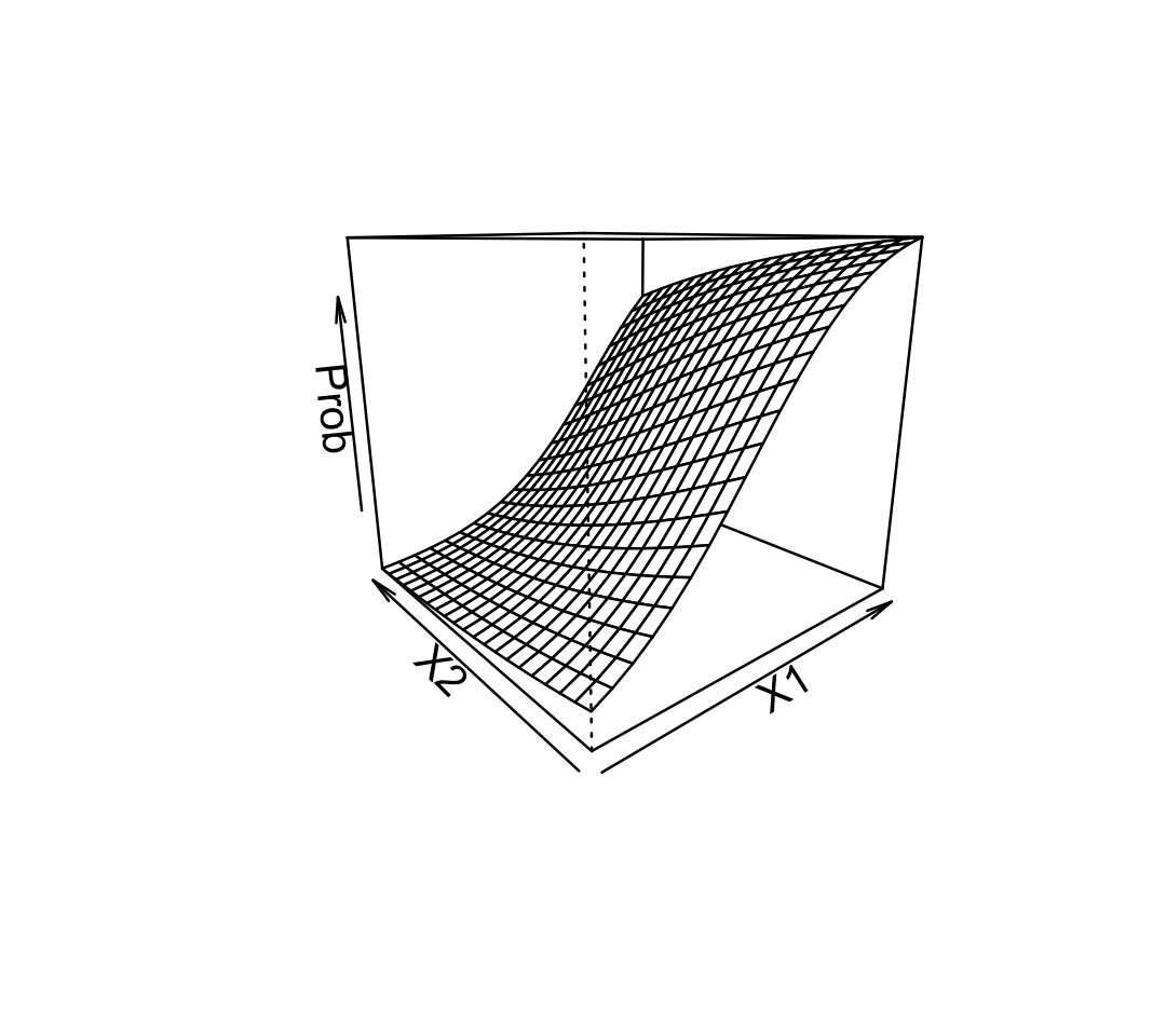
Each grid line indicates a particular fixed value of \(X_1\) or \(X_2\). Observe the shape of the lines: they curve gently, from nearly flat when the probability is close to 0 or 1 to more steeply sloped in between.
Because of this, the relationship between each predictor and the probability depends on the value of the other predictors. In this plot, for instance, a large value of \(X_1\) produces a high predicted probability—so the slope of the relationship between \(X_2\) and the probability is small. For smaller values of \(X_1\), however, the predicted probability is smaller and the slope for \(X_2\) is larger.
This nonlinearity can produce unexpected results and forces us to be very careful when interpreting logistic regression output, as we will see in Section 12.3.
When we have additional regressors, such as quadratic terms or splines, the surface can look more complicated when plotted against the original predictors—just like a linear regression with polynomial or spline terms can be nonlinear in terms of the original regressors.
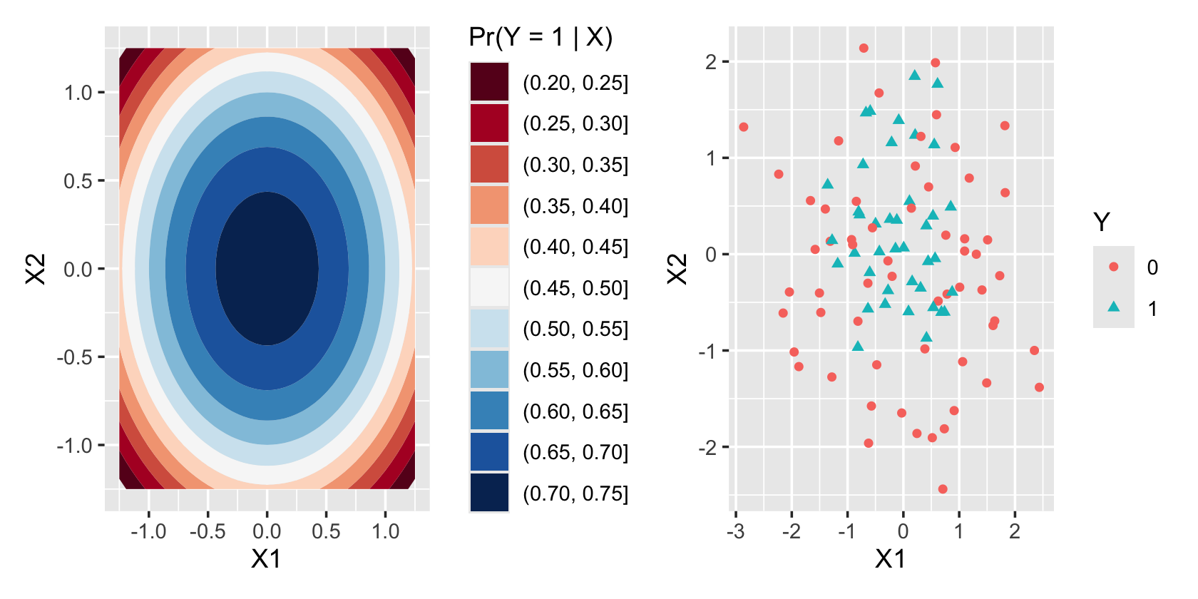
Example 12.3 (Nonlinear contours of probability) In this population, the log-odds of \(Y = 1\) change nonlinearly with \(X_1\) and \(X_2\). We can fit a polynomial model to the data:
nonlin_pop <- population(
  x1 = predictor(rnorm, mean = 0, sd = 1),
  x2 = predictor(rnorm, mean = 0, sd = 1),
  y = response(1 - 0.8 * (x1^2 + x2^2),
    family = binomial(link = "logit"))
)

nonlin_samp <- nonlin_pop |>
  sample_x(n = 100) |>
  sample_y()
Figure 12.3 illustrates the nonlinear decision boundary this produces. On the left, we see the true \(\Pr(Y = 1 \mid X_1 = x_1, X_2 = x_2)\) plotted against \(x_1\) and \(x_2\), showing the circular contour lines. On the right, we see that the \(Y = 1\) cases are concentrated toward the center of the plot, though this concentration is not as dramatic as the colorful contour plot would suggest. Reading the contour plot more carefully, we see that \(\Pr(Y = 1 \mid X)\) is above \(1/2\) for most of the plot except the outside corners, and so we’d expect to see many \(Y = 1\) cases across most of the scatterplot.
To fit a logistic regression model to this data, we could use quadratic terms in our regression, just like in a linear model. We could add these directly to our model formula or use poly() to automatically get orthogonal polynomials.
12.3 Interpretation
It might seem that logistic regression should be easy to interpret, because it gives us a model-based estimate of \(\Pr(Y = 1 \mid X = x)\) and that often is exactly the quantity we want to know. And it does so through the logit function, which gives us useful interpretations in terms of odds and log-odds. But odds and log-odds are not always easy to work with, as we will see, and it takes particular care to interpret the coefficients and predictions from a logistic model fit.
12.3.1 Log-odds, odds, and odds ratios
The first problem is that we often do not have good intuition for odds and log-odds. In a logistic fit, the so-called linear predictor is \(\beta\T X\), just as in linear regression, but that linear predictor predicts the log-odds. We must develop an intuition for log-odds values.
Exercise 12.1 (Odds, log-odds, and probabilities) For each row below, calculate the odds and log-odds that correspond to the given probability. \[\begin{align*} \Pr(Y = 1) &= 0 & \odds(Y = 1) &={} ? & \log(\odds(Y = 1)) &={} ? \\ \Pr(Y = 1) &= \frac{1}{2} & \odds(Y = 1) &={} ? & \log(\odds(Y = 1)) &={} ? \\ \Pr(Y = 1) &= 1 & \odds(Y = 1) &={} ? & \log(\odds(Y = 1)) &={} ? \end{align*}\]
Next, how do we interpret the estimated \(\hat \beta\)? From Definition 12.1, we have \[\begin{align*} \log(\odds(Y = 1 \mid X = x)) &= \beta\T x\\ \odds(Y = 1 \mid X = x) &= \exp(\beta\T x). \end{align*}\] Consequently, a one-unit increase in predictor \(X_1\) corresponds to an increase in the log-odds of \(\beta_1\): \[\begin{multline*} \log(\odds(Y = 1 \mid X_1 = \textcolor{red}{x_1 + 1}, X_2 = x_2, \dots, X_p = x_p)) -{} \\ \log(\odds(Y = 1 \mid X_1 = \textcolor{red}{x_1}, X_2 = x_2, \dots, X_p = x_p)) = \beta_1. \end{multline*}\] And this corresponds to a multiplication of the odds by \(\exp(\beta_1)\): \[\begin{align*} \frac{\odds(Y = 1 \mid X_1 = \textcolor{red}{x_1 + 1}, \dots, X_p = x_p)}{\odds(Y = 1 \mid X_1 = \textcolor{red}{x_1}, \dots, X_p = x_p)} &= \frac{\exp(\beta_1 (x_1 + 1) + \dots + \beta_p x_p)}{\exp(\beta_1 x_1 + \dots + \beta_p x_p)} \\ &= \exp(\beta_1). \end{align*}\] The quantity \(\exp(\beta_1)\) is an odds ratio (OR). It is the ratio of odds predicted with two different values of \(x_1\).
We cannot convert this to a fixed change in probability: the change in \(\Pr(Y = 1 \mid X = x)\) given a particular increase in \(x\) depends on the value of \(x\), because the conversion from odds to probability is nonlinear.
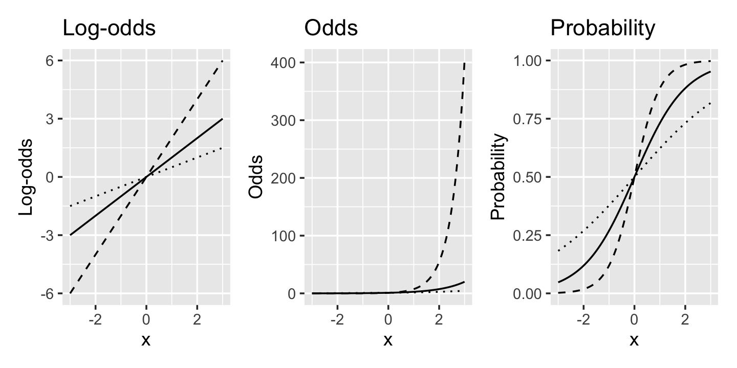
Example 12.4 (Interpreting slopes) In Figure 12.4, we’ve plotted the log-odds, odds, and probability of \(Y = 1\) for three models. All three models have \(\Pr(Y = 1 \mid X = x) = \ilogit(\beta x)\), but with three values of \(\beta\): \(\beta = (1/2, 1, 2)\). We can see that as \(x\) increases, the log-odds increase linearly while the odds are multiplied, i.e. they increase exponentially.
Example 12.5 (Diabetes in the Pima) The Pima are a Native American group who live in parts of Arizona and northwestern Mexico. After European colonization of the area displaced the Pima and forced dramatic changes to their way of life, the Pima people developed rates of type 2 diabetes among the highest in the world. The group has hence been studied by the National Institute of Diabetes and Digestive and Kidney Diseases since 1965 (Smith et al. 1988).
The MASS package contains two data frames, Pima.tr and Pima.te, containing observations from this data. Each observation represents one Pima woman, at least 21 years old, who was tested for diabetes as part of the study. The type column indicates if they had diabetes according to the diagnostic criteria. We will use the Pima.tr dataset and explore relationships between various predictors and diabetes.
First, we can load the package and check how the type factor is ordered. We see that "No" is the first level, so glm() will model the probability of the second level, "Yes". This means our model will be for the probability of diabetes, which is probably the most intuitive option.
library(MASS)

levels(Pima.tr$type)
[1] "No" "Yes"To demonstrate the interpretation of the model, let’s make a model using a binary factor variable and a continuous variable. The data contains a column npreg for the number of pregnancies, so let’s make a factor indicating whether the patient has had any pregnancies, then fit a model using that and diastolic blood pressure as predictors. (Yes, Exercise 9.2 showed the danger of dichotomizing predictors and throwing away information; but we are only doing this to demonstrate how to interpret coefficients.)
# ggeffects requires factors, not logicals
Pima.tr$pregnancy <- factor(
  ifelse(Pima.tr$npreg > 0, "Yes", "No")
)

pima_fit <- glm(type ~ pregnancy + bp, data = Pima.tr,
family = binomial())| Term | Estimate | SE | \(\exp(\text{Estimate})\) | z | p |
|---|---|---|---|---|---|
| (Intercept) | -3.165 | 1.077 | 0.042 | -2.939 | 0.003 |
| pregnancyYes | -0.468 | 0.427 | 0.626 | -1.097 | 0.273 |
| bp | 0.040 | 0.014 | 1.041 | 2.886 | 0.004 |
Table 12.1 shows the estimates from this model. Let’s see how to interpret the estimates; we’ll discuss the standard errors and test statistics in Section 12.6.
Going through the terms in turn,
- Intercept: We estimate that the log-odds of diabetes for a Pima woman who has never been pregnant and has a diastolic blood pressure of 0 (!) are -3.2, so the odds are 0.0422.
- Pregnancy: Pregnancy changes the log-odds of diabetes, relative to the baseline value, by -0.47. The odds ratio is 0.626, i.e. pregnancy multiplies the odds of pregnancy by 0.626.
- Blood pressure: Each unit of increase in blood pressure (measured in mm Hg) is associated with an increase in the log-odds of diabetes of 0.04, or a multiplication of the odds of diabetes by 1.04.
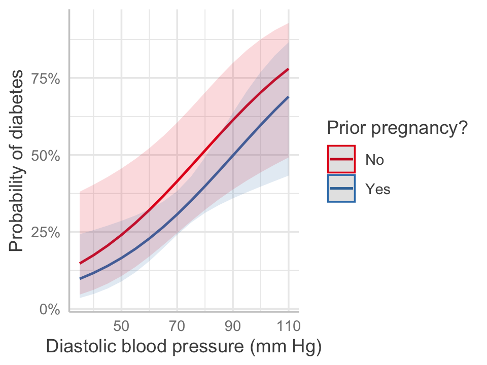
We can construct an effect plot (Section 7.7) as usual, as shown in Figure 12.5. The plot converts back to predicted probability of diabetes, showing the nonlinear relationship inherent to the logit transformation. Notice how the gap between the two lines—for women with and without a prior pregnancy—is not constant across the range of blood pressures. The odds ratio is constant, because there is no interaction here, but the difference in probability is not.
12.3.2 Case–control and cohort studies
One common use for logistic regression is modeling how a binary outcome is associated with different exposure variables. For example, we might want to know what risk factors are associated with a particular disease. We could imagine several ways to do this:
- Prospective cohort study: We take a random sample of healthy people from the population. We follow this cohort over many years, recording data about the risk factors they are exposed to during this time, and then record whether they have been diagnosed with the disease by the end of the study period.
- Retrospective cohort study: We take a random sample from the population. Some of the sampled people have the disease, others do not. We ask them about the risk factors they were exposed to.
- Case–control study: We sample \(n\) people from the population who have the disease (the cases), and a similar number of people from the population who do not (the controls). We ask them about the risk factors they were exposed to.
These are very different study designs, and they may make sense in different circumstances. A prospective cohort study seems most desirable, since we can collect very detailed data about each person as they are exposed to the risk factors, and see who develops the disease—but depending on the disease, such a study may take decades to yield useful data. We’d be sitting around for years just waiting for some of the people to develop the disease.
A retrospective cohort study avoids this problem, but limits the exposure data we can collect (because we have to ask about the past, and there may not be detailed records of past exposures). It also is very difficult to do for rare diseases: if an illness only affects 0.1% of the population, we’d require a sample of thousands of people just to get a few people with the disease. If gathering the data requires extensive questionnaires and medical tests, such a study could be impracticably expensive and time-consuming.
The case–control study avoids that problem. We can find people with the disease—perhaps through a hospital or through a patient support organization—and recruit a sample of them, then recruit a sample of control people who are similar to the patients but do not have the disease. We still have to get the exposure data retrospectively, but obtaining enough patients may be much easier than in a retrospective cohort study.
| Exposure | No disease | Disease | Total |
|---|---|---|---|
| Not exposed | \(\gamma_{00}\) | \(\gamma_{01}\) | \(\gamma_{0.}\) |
| Exposed | \(\gamma_{10}\) | \(\gamma_{11}\) | \(\gamma_{1.}\) |
| Total | \(\gamma_{.0}\) | \(\gamma_{.1}\) | 1 |
Consider the population proportions shown in Table 12.2 for the case when we have a binary exposure and binary outcome. In a cohort study, we obtain a random sample from the population, so we can estimate these proportions, and we could estimate the relative risk: \[ \text{RR} = \frac{\Pr(\text{disease} \mid \text{exposed})}{\Pr(\text{disease} \mid \text{not exposed})} = \frac{\gamma_{11} / \gamma_{1.}}{\gamma_{01} / \gamma_{0.}}. \] The relative risk directly answers the question “How many times more likely am I to develop the disease if I am exposed, compared to if I’m not exposed?” It is on the probability scale, so if the relative risk is 3 and the probability of getting the disease when not exposed is 10%, the probability if you’re exposed is 30%.
Let \(X_{00}, X_{01}, X_{10}, X_{11}\) denote the number of patients in each category that we observe in our study. In a cohort study, \[ X_{00}, X_{01}, X_{10}, X_{11} \sim \multinomial(n, (\gamma_{00}, \gamma_{01}, \gamma_{10}, \gamma_{11})), \] and so we can simply estimate \[ \widehat{\text{RR}} = \frac{X_{11} / (X_{10} + X_{11})}{X_{01} / (X_{00} + X_{01})}. \]
But in a case–control study, this will not work. We deliberately sample a certain number of cases and a certain number of controls, so instead of multinomial sampling, we have \[\begin{align*} X_{11} &\sim \binomial(n_\text{case}, \Pr(\text{exposed} \mid \text{disease})) \\ X_{10} &\sim \binomial(n_\text{control}, \Pr(\text{exposed} \mid \text{no disease})), \end{align*}\] where \(n_\text{case}\) and \(n_\text{control}\) are chosen as part of the study design. (Consequently, \(X_{00} = n_\text{control} - X_{10}\) and \(X_{01} = n_\text{case} - X_{11}\).)
We can estimate the binomial proportions easily enough; for example, we can estimate \(\Pr(\text{exposed} \mid \text{disease})\) using \(X_{11} / (X_{01} + X_{11})\). We can also note that the odds ratio for exposure is \[ \frac{\odds(\text{exposed} \mid \text{disease})}{\odds(\text{exposed} \mid \text{no disease})} = \frac{\gamma_{11} / \gamma_{01}}{\gamma_{10} / \gamma_{00}} = \frac{\gamma_{11} \gamma_{00}}{\gamma_{10} \gamma_{01}}, \] and again, we can estimate these odds for the same reason we can estimate the proportions. But it also turns out that \[ \text{OR} = \frac{\odds(\text{disease} \mid \text{exposed})}{\odds(\text{disease} \mid \text{not exposed})} = \frac{\gamma_{11} / \gamma_{10}}{\gamma_{01} / \gamma_{00}} = \frac{\gamma_{11} \gamma_{00}}{\gamma_{10} \gamma_{01}}. \] The odds ratio we want is the same as the odds ratio we can estimate given the sample design! A procedure that estimates odds ratios given the case–control data, like a logistic regression, will give estimates of the correct odds ratio, even though we have not drawn a simple random sample of the population.
Because of this useful property of odds ratios, case–control studies are widely used in medicine, epidemiology, nutrition, and related fields, and logistic regression is widely used to interpret case–control study results. Their crucial advantage is the ability to estimate odds ratios despite deliberately sampling a specific proportion of cases and controls; their crucial weakness is the inability to estimate relative risks. Also, many people treat the words “odds” and “probability” as interchangeable, and hence do not realize that odds ratios and relative risks are different things. This can lead to serious misinterpretations of results.
12.4 Properties of the estimator
In linear regression, Theorem 5.4 told us that \(\hat \beta\) is unbiased, has a variance we can calculate, and is normally distributed when certain conditions are true. We can make similar claims for logistic regression, but proving them is less straightforward, and the claims will only be asymptotically true as \(n \to \infty\).
12.4.1 Sampling distribution of estimates
To begin, we make use of a general property of maximum likelihood estimators.
Theorem 12.1 (Asymptotic distribution of MLEs) Let \(X_1, X_2, \dots, X_n\) be iid draws from a distribution parameterized by \(\theta \in \R^p\). Let \(\hat \theta\) be the MLE for \(\theta\). Under certain regularity conditions on the distribution, \[ \sqrt{n}(\hat \theta - \theta) \convd \normal(0, I(\theta)^{-1}), \] where \(I(\theta)\) is the Fisher information matrix. The Fisher information is defined to be the matrix with elements \[ I_{i,j}(\theta) = \cov\left(\frac{\partial}{\partial \theta_i} \ell(\theta), \frac{\partial}{\partial \theta_j} \ell(\theta) \right), \] and when regularity conditions hold—such as with exponential dispersion families—we can write this in terms of the Hessian: \[ I(\theta) = - \E[D^2 \ell(\theta)]. \]
Proof. Schervish (1995), definition 2.79, proposition 2.84, and theorem 7.57.
Conveniently, the binomial distribution is an exponential family distribution; and even more conveniently, the iteratively reweighted least squares procedure of Section 12.2.1 provides a natural way to calculate the Fisher information, because \(\E[D^2 \ell(\beta)] = -\X\T W \X\). Hence the maximum likelihood estimates of \(\beta\) in logistic regression are asymptotically unbiased and have an asymptotic normal distribution whose variance we can estimate as \[ \widehat{\var}(\hat \beta) = (\X\T W \X)^{-1}. \] These variances are automatically estimated by R and used to produce the standard errors it reports for logistic regression models.
12.4.2 The likelihood and the deviance
In linear regression, we used the residual sum of squares (RSS) as the basis for several measures of fit. The RSS is itself interpretable: an RSS of 0 means the model predicts perfectly, and is the best possible RSS; we can divide a nonzero RSS by \(n - p\) to get an estimate of the variance \(\sigma^2\); and we can use the difference in RSS between two nested models as the basis for an \(F\) test. You may also be familiar with goodness-of-fit metrics like \(R^2\) that are based on the RSS.
In logistic regression, the RSS is less meaningful. Instead we define the deviance as a measure of model fit.
Definition 12.3 (Deviance) Let \(\ell(\hat \beta)\) be the log-likelihood function for the chosen model, evaluated at the fitted \(\hat \beta\). The deviance or residual deviance is \[ \dev = 2 \ell_\text{sat} - 2 \ell(\hat \beta), \] where \(\ell_\text{sat}\) is the log-likelihood for a saturated model. A saturated model is one where \(\hat y_i = y_i\) for every observation \(i\). A small deviance implies a model that fits nearly as well as the saturated model.
An alternative definition makes clear the contribution of individual terms. Let \(\ell(\hat y; y)\) be the log-likelihood for a model that predicts \(\E[Y \mid X] = \hat y\). Then \(\ell_\text{sat} = \ell(y; y)\), and the deviance for a particular model can be written as \[\begin{align*} \dev &= 2 \ell(y; y) - 2 \ell(\hat y; y) \\ &= 2 \sum_{i=1}^n \left(\ell(y_i; y_i) - \ell(\hat y_i; y_i)\right). \end{align*}\]
The deviance is automatically reported by the summary() function for logistic regression fits, along with a null deviance, which is the deviance of a null model that only contains an intercept term. For a particular dataset, the deviance is hence bounded between 0 (perfect fit) and the null deviance,2 giving you a sense of scale for how much your model improves on a null model and how far from perfect it is.
Example 12.6 (Saturated model in logistic regression) The notion of a “saturated” model is often confusing. In logistic regression, the saturated model is a model that predicts \(\Pr(Y_i = 1 \mid X_i = x_i) = 1\) for observations where the observed \(y_i = 1\), and vice versa for \(y_i = 0\). From the log-likelihood defined above, we can write the saturated model’s log-likelihood as \[\begin{align*} \ell(\beta) &= \sum_{i=1}^n y_i \log(\Pr(y_i = 1 \mid X_i = x_i)) + (1 - y_i) \log(\Pr(y_i = 0 \mid X_i = x_i)) \\ &= y_i \log(1) + (1 - y_i) \log(1) \\ &= 0. \end{align*}\] (It seems odd to have both \(\Pr(y_i = 1 \mid X_i = x_i)\) and \(\Pr(y_i = 0 \mid X_i = x_i)\) be \(1\) for a particular \(i\), but recall the likelihood was written as a product as a way to write the likelihood was either of those probabilities, depending on if \(y_i = 0\) or \(y_i = 1\). We could equivalently write this as a sum of terms, each of which only involves one or the other case, based on the observed data.)
Yes, the log-likelihood of the saturated model is zero, because the saturated model assigns probability 1 to each observation. This is a result peculiar to logistic regression; in other generalized linear models, rather than binary outcomes we may have a range of discrete or continuous outcomes, and the stochastic term of the assumed model cannot assign probability 1 to a particular outcome. (For example, if \(Y \sim \poisson(7)\), we do not have \(\Pr(Y = 7) = 1\).) We will see this in more detail in Example 13.8.
12.5 Assumptions and diagnostics
As we saw in Definition 12.1, logistic regression makes two basic assumptions about the population relationship:
- The log-odds is linearly related to the regressors: \(\log(\odds(Y = 1 \mid X = x)) = \beta\T x\).
- The observations \(Y_i\) are conditionally independent given the covariates \(X_i\).
To evaluate if these assumptions are suitable in a particular situation and detect problems with fitted models, we need exploration and diagnostic tools.
12.5.1 Exploratory visualization
In linear regression, we generally make scatterplots of the predictors versus the response to judge the shape of the relationship, before moving on to modeling and diagnostics. That’s harder in logistic regression because of the binary response, but it’s still possible if you’re creative.
Plotting a predictor versus \(Y\) directly is rarely useful because the scatterplot makes it very difficult to judge the rate of \(Y = 1\) observations, as we saw in the left panel of Figure 12.2. However, if we bin the predictor and plot the fraction of observations with \(Y = 1\) in each bin, we can see the trend more clearly.
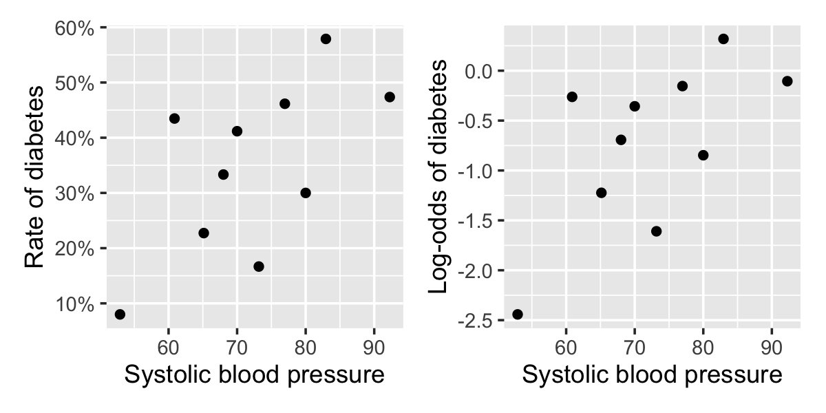
Example 12.7 (EDA in the Pima data) In the Pima diabetes data from Example 12.5, it would be useful to plot the relationship between blood pressure and diabetes first, so we can judge whether blood pressure should be included in the model as-is or if additional nonlinear terms are needed.
We can break blood pressure up into 10 bins, calculate the percentage of people with diabetes in each bin, and plot this. The relationship will be nonlinear, since the covariates are never linearly related to the probability, so we can also transform the probabilities to log-odds.
The regressinator provides a bin_by_quantile() function to break data up into bins using a variable and the empirical_link() function to automatically transform the average of a variable onto the link scale. This integrates well with dplyr’s grouping: bin_by_quantile() splits the data into groups, and empirical_link() can be used inside summarize() to make a column.
library(regressinator)
library(dplyr)

rate_by_bp <- Pima.tr |>
  mutate(diabetes = (type == "Yes")) |>
  bin_by_quantile(bp, breaks = 10) |>
  summarize(
    mean_bp = mean(bp),
    prob = mean(diabetes),
    log_odds = empirical_link(
      diabetes,
      family = binomial(link = "logit")),
    n = n()
  )
Of course, this can also be calculated without dplyr, for instance by looping through ranges of blood pressures and calculating averages by subsetting the data. In any case, the result is plotted in Figure 12.6. The relationship is not strong—there is a lot of variation in diabetes rate from bin to bin—but it is at least not obviously nonlinear.
This is called an empirical logit plot when done for logistic regression. As it can be done for any link function, I call it an empirical link plot, though this name is not widely used (since people often skip exploratory plots for binary outcomes).
These plots serve the same role as scatterplots of the data in ordinary linear regression, helping us choose the appropriate model. But to tell if our selected model behaves as it should, we need residual diagnostics.
12.5.2 Conventional residuals
As we mentioned earlier, many of the nice geometric features of linear regression do not apply to logistic regression. This particularly applies to residuals, which were easy to work with in linear regression (see Section 5.5) but are particularly inconvenient here. Let’s define basic residuals and explore their properties.
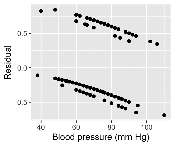
Definition 12.4 (Logistic regression residuals) Let \(\hat y_i = \ilogit(\hat \beta\T x_i)\), the predicted probability for observation \(i\). Then the residual is \[ \hat e_i = y_i - \hat y_i. \]
In R, the residuals() method for generalized linear models can provide multiple types of residuals. By specifying type = "response", we can get the residuals of Definition 12.4.
Because \(y_i \in \{0, 1\}\), the residual \(\hat e_i\) can only take on two possible values when we condition on a particular value \(x_i\). This makes plots of the residuals versus the predictors hard to interpret directly. For example, Figure 12.7 shows the residuals for the model fit in Example 12.5, which show a striped pattern.
These residuals can be standardized to have constant variance; while this does not make them any easier to interpret for logistic regression, we will find uses for standardized residuals with other generalized linear models, so we may as well define them now.
Definition 12.5 (Logistic regression standardized residuals) The standardized residuals are defined to be \[ r_i = \frac{\hat e_i}{\sqrt{\widehat{\var}(y_i)}}, \] where \(\widehat{\var}(y_i)\) is the estimated variance of the response. In logistic regression, because the variance of a \(\bernoulli(p)\) random variable is \(p (1 - p)\), \(\widehat{\var}(y_i) = \hat y_i (1 - \hat y_i)\), with \(\hat y_i\) defined as in Definition 12.4. The standardized residuals are then \[ r_i = \frac{\hat e_i}{\sqrt{\hat y_i (1 - \hat y_i)}}. \]
The standardized residuals are sometimes known as the Pearson residuals.
Another similar residual definition is the deviance residuals. In Definition 12.3, we redefined the deviance in terms of a sum over all observations, and so we can use the contribution from each observation to define a deviance.
Definition 12.6 (Deviance residuals) The deviance residuals are defined to be \[ d_i = \sign(y_i - \hat y_i) \sqrt{2 \left(\ell(y_i; y_i) - \ell(\hat y_i; y_i)\right)}, \] where \(\ell\) and \(\hat y_i\) are defined as in Definition 12.3.
The use of the sign of the difference ensures that the deviance residuals are positive when the observation is larger than predicted, and negative when the observation is smaller, just as with ordinary residuals.
For both standardized residuals and deviance residuals, it is tempting to think that the residuals must be approximately normally distributed in a well-specified model. That is not true for logistic regression, for reasons that Figure 12.7 should make clear. Residual Q-Q plots and other checks are not appropriate here, although we will see later that they sometimes can be for other generalized linear models.
In R, the residuals() method for GLMs supports a type argument, so you can select type = "deviance" (deviance residuals), type = "response" (ordinary residuals), or type = "pearson" (standardized residuals). The broom package’s augment() method for GLMs similarly supports a type.residuals argument to specify either deviance or Pearson (standardized) residuals.
12.5.3 Partial residuals
As in linear regression (Definition 7.2), we can define partial residuals.
Definition 12.7 (Partial residuals for GLMs) Consider a model such that \(g(\E[Y \mid X = x]) = \eta(x)\), so that \(\hat y_i = g^{-1}(\hat \eta(x_i))\). (For example, in logistic regression, \(g\) is the logit function, \(\eta(x) = \beta\T x\), and \(\hat y_i\) is the predicted probability.)
Select a focal predictor \(X_f\) and write \(\eta\) as \(\eta(X_f, X_o)\), where \(X_o\) represents all predictors except the focal predictor.
The partial residual for observation \(i\) is \[\begin{align*} r_{if} &= \left(y_i - \hat y_i\right) g'(\hat y_i) + \left(\hat \eta(x_{if}, 0) - \hat \beta_0 \right) \\ &= \hat e_i g'(\hat y_i) + \left(\hat \eta(x_{if}, 0) - \hat \beta_0 \right), \end{align*}\] where \(\hat e_i\) is the residual defined in Definition 12.4, \(\hat \beta_0\) is the intercept of \(\hat \eta(x)\), and \[ g'(\hat y_i) = \frac{\partial}{\partial \hat y_i} g(\hat y_i). \]
Notice the parallel to Definition 7.2: this is almost the same as partial residuals in linear regression, except we include the derivative of the link function \(g\).
The simple interpretation is this: We Taylor-expand the nonlinear link function around \(\hat y_i\) and take the first term, \((y_i - \hat y_i) g'(\hat y_i)\). The link transforms from response scale (\(y\)) to link scale (log-odds), so this produces an approximate residual on the log-odds scale. We then convert this to a partial residual on the log-odds scale using \(\hat \eta(x_{if}, 0)\). We have to use a Taylor expansion because we can’t transform directly: \(g(y_i) = \pm \infty\), so \(g(y_i) - g(\hat y_i)\) would not be a useful residual.
This suggests the partial residuals are essentially those of a linear approximation to the logistic regression. That is true: they’re the same partial residuals we’d get from the last step of iteratively reweighted least squares (Section 12.2.1). In IRLS, the solution for the final update of \(\hat \beta\) is \[ \hat \beta^{(n + 1)} = (\X\T W \X)^{-1} \X\T W Z^{(n)}, \] where \(Z^{(n)} = \X \hat \beta^{(n)} + W^{-1} (\Y - P)\), \(P\) is a vector whose entries are the estimates of \(\Pr(Y = 1 \mid X = x)\), and \(W\) is a diagonal matrix whose diagonal entries are \(P_i(1 - P_i)\). Again, by analogy to linear regression, this is like a weighted least squares fit to predict \(Z^{(n)}\) from \(\X\) using the weights \(W\). The residuals of such a fit would be \(Z^{(n)} - \X \hat \beta^{(n + 1)}\); when IRLS has converged, \(\hat \beta^{(n + 1)} \approx \hat \beta^{(n)}\), so the residuals are approximately \(W^{-1} (\Y - P)\).
Let’s now consider what these residuals would be in the case of logistic regression. Note that \(P_i = \hat y_i\), so the entries of the residual vector are \[ r_i = (y_i - \hat y_i) / W_{ii} = \frac{y_i - \hat y_i}{\hat y_i (1 - \hat y_i)}. \] Compare that to the first term in the partial residual definition. For logistic regression, \[ g'(\hat y_i) = \frac{\partial}{\partial \hat y_i} \logit(\hat y_i) = \frac{1}{\hat y_i (1 - \hat y_i)}, \] so the first term is the same as \(r_i\)!
Consequently, the partial residuals for logistic regression (as defined in Definition 12.7) are the same as the partial residuals for linear regression (as defined in Definition 7.2) from the regression fit on the last iteration of IRLS. And so we can see partial residuals in logistic regression as being partial residuals for a linear approximation to the nonlinear fit, and they inherit some of the useful properties of partial residuals in linear fits (Cook and Croos-Dabrera 1998; Landwehr et al. 1984). In particular, we can see the shape of the partial residual plots as illustrating the shape of the relationship between the predictor and log-odds, subject to the accuracy of the linearization—so the shape is locally accurate, but may not be so accurate if the response probabilities cover a wide range over which the logit is not very linear.
We can combine partial residuals with another trick—smoothing—to detect misspecification in model fits. Smoothing is necessary because in logistic regression, the individual residuals are not very informative, but trends in their mean can be. This makes it particularly difficult to detect misspecification when our sample size is small, but we have better chances when there is enough data for the smoothed trends in residuals to be meaningful.
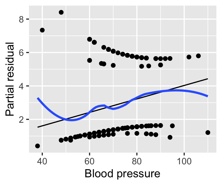
Example 12.8 (Partial residuals from the Pima data) The regressinator’s partial_residuals() function, introduced in Example 9.3, also supports partial residuals for models fit with glm(). Figure 12.8 shows the partial residuals for the blood pressure predictor from the model fit in Example 12.5. (It does not make sense to calculate partial residuals for the pregnancy predictor, as it is a factor variable.) The smoothing line helps the interpretation by revealing deviations from the predicted effects, though these residuals are still somewhat difficult to interpret visually.
12.5.4 Randomized quantile residuals
Residuals are so troublesome in logistic regression because \(Y\) is discrete and residuals can only take on specific values. Dunn and Smyth (1996) proposed a solution to make more useful residuals: transform them to have a continuous, not discrete, distribution. This requires randomization, so the resulting residuals are called randomized quantile residuals. These can be defined generally for any regression model with independent responses, regardless of the particular distribution assumed for \(Y\).
Definition 12.8 (Randomized quantile residuals) Let \(F_Y(y; x, \beta)\) be the predicted cumulative distribution function of \(Y \mid X = x\). When \(F_Y\) is a continuous distribution, the randomized quantile residual for observation \(i\) is \[ r_{q,i} = F_Y(y_i; x_i, \hat \beta). \] When \(F_Y\) is a discrete distribution, let \[\begin{align*} a_i &= \lim_{y \uparrow y_i} F_Y(y; x_i, \hat \beta), & b_i &= F_Y(y_i; x_i, \hat \beta) \end{align*}\] and draw \[ r_{q,i} \sim \uniform(a_i, b_i). \]
In logistic regression, of course, \(y_i \in \{0, 1\}\), so this can be simplified. The cumulative distribution function is shown in Figure 12.9. As shown in the figure, we can write it as \[\begin{align*} F_Y(0; x_i, \hat \beta) &= \widehat{\Pr}(Y = 0 \mid X = x_i)\\ &= 1 - \ilogit(\hat \beta\T x_i)\\ F_Y(1; x_i, \hat \beta)&= 1. \end{align*}\]
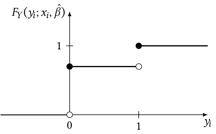
Consequently, the randomized quantile residual is \[ r_{q,i} \sim \begin{cases} \uniform(0, 1 - \ilogit(\hat \beta\T x_i)) & \text{when $y_i = 0$}\\ \uniform(1 - \ilogit(\hat \beta\T x_i), 1) & \text{when $y_i = 1$.} \end{cases} \]
Theorem 12.2 (Distribution of randomized quantile residuals) When the model is correct, the randomized quantile residuals are \(\uniform(0, 1)\).
Proof. It is easiest to see this through the density of \(r_{q,i}\). We can write it as a mixture of two densities, for \(y_i = 0\) and \(y_i = 1\): \[\begin{multline*} f_R(r_{q,i} \mid X_i = x_i) = f_R(r_{q,i} \mid X_i = x_i, Y_i = 0) \Pr(Y_i = 0 \mid X_i = x_i) + {}\\ f_R(r_{q,i} \mid X_i = x_i, Y_i = 1) \Pr(Y_i = 1 \mid X_i = x_i). \end{multline*}\] These two densities have disjoint support: one is supported on \([0, 1 - \ilogit(\hat \beta\T x_i)]\), the other on \([1 - \ilogit(\hat \beta\T x_i), 1]\). Consequently, the density is \[\begin{align*} f_R(r_{q,i} \mid X_i = x_i) &= \begin{cases} \frac{1}{1 - \ilogit(\hat \beta\T x_i)} \Pr(Y_i = 0 \mid X_i = x_i) & \text{when $y_i = 0$}\\ \frac{1}{\ilogit(\hat \beta\T x_i)} \Pr(Y_i = 1 \mid X_i = x_i) & \text{when $y_i = 1$.} \end{cases}\\ &= \begin{cases} \frac{1}{\widehat{\Pr}(Y_i = 0 \mid X_i = x_i)} \Pr(Y_i = 0 \mid X_i = x_i) & \text{when $y_i = 0$} \\ \frac{1}{\widehat{\Pr}(Y_i = 1 \mid X_i = x_i)} \Pr(Y_i = 1 \mid X_i = 1) & \text{when $y_i = 1$.} \end{cases} \end{align*}\] These two densities are equal to 1 when \(\Pr(Y_i = y_i \mid X_i = x_i) = \widehat{\Pr}(Y_i = y_i \mid X_i = x_i)\). A density of 1 between 0 and 1 is the density of a \(\uniform(0, 1)\).
Because of this property, we can use plots of randomized quantile residuals against predictors and fitted values, as with any other residuals, to check the fit of our model. It is also useful to check that their distribution is indeed uniform (e.g., with a Q-Q plot).3 When the model is incorrectly specified, the distribution will not be uniform, producing patterns on the residual plots that can be interpreted.
Example 12.9 (Randomized quantile residuals from the Pima data) In R, the DHARMa package implements randomized quantile residuals. Upon loading the package, we use simulateResiduals() to do the necessary simulation, and the residuals() method for the resulting object retrieves the randomized quantile residuals. Alternately, the regressinator provides the augment_quantile() function to augment the model fit with randomized quantile residuals:
library(DHARMa)
dh <- simulateResiduals(pima_fit)
pima_aug <- augment(pima_fit) |>
mutate(.quantile.resid = residuals(dh))
# or, equivalently:
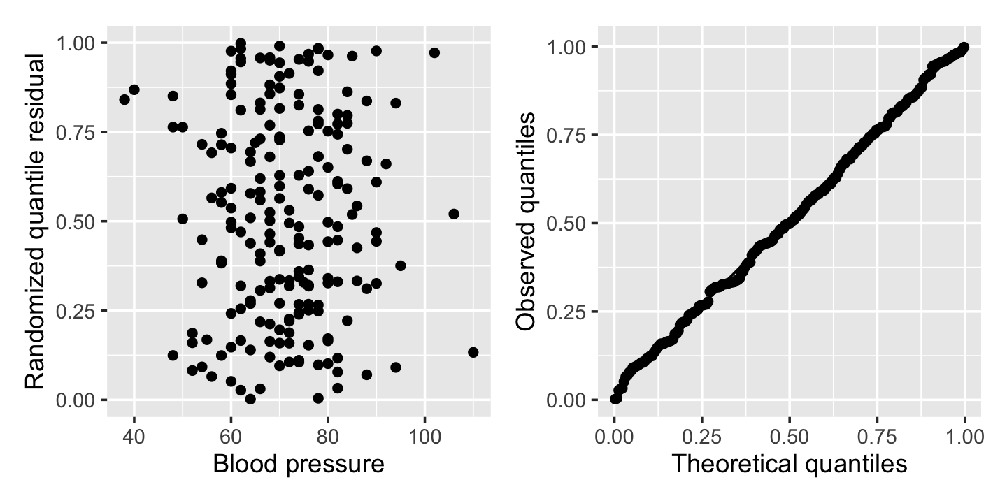
pima_aug <- augment_quantile(pima_fit)It is helpful to plot these residuals against the predictors or fitted values, as with other residuals, and it is also helpful to verify their distribution is uniform. Figure 12.10 shows the residuals from Example 12.5 plotted against blood pressure, as well as a Q-Q plot comparing them to the uniform distribution. No obvious problems appear: the residuals appear extremely uniform, and they appear as a uniform blob when plotted against the predictor.
(Note that DHARMa is designed to work with many types of models, including those where the response distribution is not easily defined analytically. Rather than hardcoding \(F_Y\) for different types of models, it obtains it empirically by simulating many observations from the fitted model. This makes the residuals slower to calculate than you might expect, but allows us to use randomized quantile residuals in many unusual settings.)
We’ll return to randomized quantile residuals in Section 13.7, when we apply them to other generalized linear models and explore examples of different kinds of model misspecification.
12.5.5 Calibration
Besides residuals, another useful diagnostic for logistic regression models is calibration. Roughly speaking, a calibrated model is one whose predicted probabilities are accurate: if it predicts \(\Pr(Y = 1 \mid X = x) = 0.8\) for a particular \(x\), and we observe many responses with that \(x\), about 80% of those responses should be 1 and 20% should be 0.
If we are lucky enough to have a dataset where the same \(x\) appears a hundred times, it would be fairly easy to check calibration. Unfortunately this does not often happen.4 When we have continuous predictors, we usually do not see exact repeat values, and so we do not see observations with exactly the same predicted probabilities.
We can instead approximate: for observations with \(\Pr(Y_i = 1 \mid X_i = x_i) \approx 0.8\), for some definition of \(\approx\), what fraction have \(Y_i = 1\)? One simple way to check this is a calibration plot.
Definition 12.9 (Calibration plot) For a model that predicts the probability of a binary outcome, a calibration plot is a plot with the model’s fitted probabilities on the \(X\) axis and the observed \(Y\) on the \(Y\) axis, smoothed using an appropriate nonparametric smoother.
Smoothing the response makes sense because a nonparametric smoother essentially takes the local average of \(Y\), and in a binary problem the local average is essentially the local fraction of responses with \(Y = 1\). Ideally, then, a calibration plot would be a perfect diagonal line, so that the fitted probability and observed fraction are always equal.
Example 12.10 (A sample calibration plot) Let’s revisit Example 12.5 and produce a calibration plot for our original fit. Notice that we convert the response from a factor to 0 or 1, so the smoother can take the average. The calibration looks good across most of the range, but as the predicted probability gets over 0.6, we see odd behavior; examining the plotted points, it appears this is due to a few observations with high predicted probability but \(Y = 0\). We should not get too worried over two or three observations, so this is not particularly concerning.
calibration_data <- data.frame(
  x = predict(pima_fit, type = "response"),
  y = ifelse(Pima.tr$type == "Yes", 1, 0)
)

ggplot(calibration_data, aes(x = x, y = y)) +
  geom_point() +
  geom_smooth(se = FALSE) +
  geom_abline(slope = 1, intercept = 0, linetype = "dashed") +
  labs(x = "Predicted probability", y = "Observed fraction") +
  ylim(0, 1)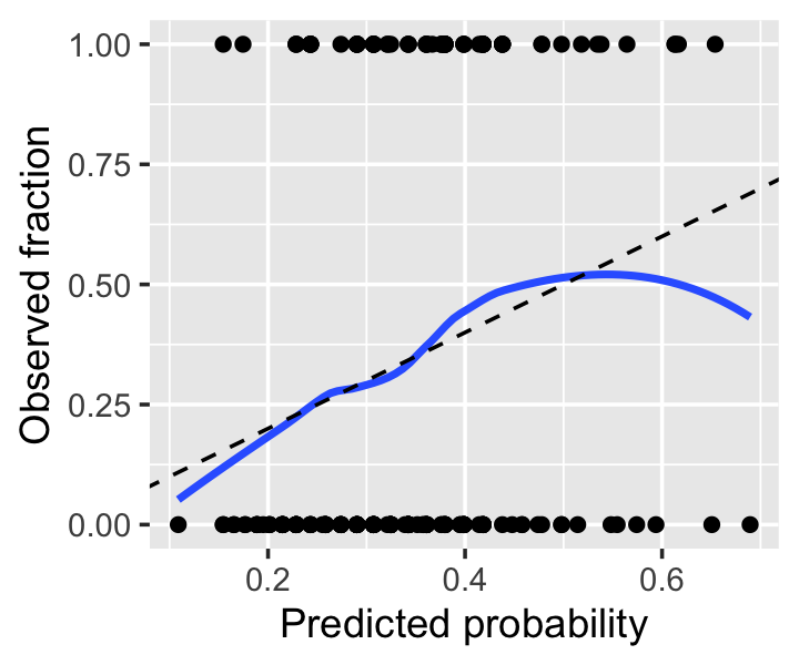
pima_fit.
The Hosmer–Lemeshow test takes this idea and turns it into a goodness-of-fit test, by comparing predicted to observed probabilities at different points and combining them to produce a test statistic whose distribution can be approximated under the null hypothesis that the fitted model is correct (Hosmer et al. 2013, sec. 5.2.2). You will often see this test used by applied scientists, who appreciate having a single test that (ostensibly) tells them if their model is good.
But perfect calibration does not make a good model. Suppose we obtain a particular dataset where \(Y = 1\) about 50% of the time. We could fit a model that predicts \(\Pr(Y = 1 \mid X = x) = 0.5\) for all \(x\). This model would be perfectly calibrated, but it would not be particularly good at predicting. Calibration hence should be used together with other measures of the adequacy of the model fit, not on its own.
Conversely, poor calibration does not itself tell us how to improve a model. Residuals, partial residuals, and related diagnostics can give us better ideas of how to improve our fits. Calibration is merely one tool, not a one-stop test for everything.
12.6 Inference
Inference for logistic regression is similar to inference for linear regression, except we must use Theorem 12.1 to estimate \(\widehat{\var}(\hat \beta)\), and \(\hat \beta\) is only asymptotically normally distributed (as \(n \to \infty\)) rather than having an exact normal distribution (if the errors are normally distributed).
12.6.1 Wald tests
Analogously to Theorem 5.6, we can define tests for individual coefficients or linear combinations thereof.
Theorem 12.3 (Wald tests) When \(\hat \beta\) is estimated using maximum likelihood and the model is correct, \[ z = \frac{\hat \beta_i - \beta_i}{\sqrt{\widehat{\var}(\hat \beta_i)}} \convd \normal(0, 1) \] as \(n \to \infty\). The statistic \(z\) is called the Wald statistic (for Abraham Wald), and can be used to test null hypotheses of the form \(H_0 : \beta_i = c\) by substituting \(c\) for \(\beta_i\).
More generally, for any fixed \(a \in \R^p\), \[ \frac{a\T \hat \beta - a\T \beta}{\sqrt{a\T \widehat{\var}(\hat \beta) a}} \convd \normal(0, 1). \] This test statistic can be used to test null hypotheses of the form \(H_0: a\T \beta = c\) by substituting \(c\) for \(a\T \beta\).
To implement a Wald test ourselves, we can use vcov() to get the estimated variance matrix (which R produces from IRLS).
12.6.2 Confidence intervals
To form confidence intervals for parameters (or linear combinations of them), we can invert a Wald test. An approximate \(1 - \alpha\) confidence interval for \(\beta_i\) is hence \[ \left[ \hat \beta_i + z_{\alpha/2} \sqrt{\widehat{\var}(\hat \beta_i)}, \hat \beta_i + z_{1 - \alpha/2} \sqrt{\widehat{\var}(\hat \beta_i)} \right], \] where \(z_\alpha\) denotes the \(\alpha\) quantile of the standard normal distribution. The approximation is good when the sample size is large and the distribution of \(\hat \beta\) is approximately normal.
One particular linear combination of the parameters is the fitted linear predictor \(\hat \beta\T X\). We can use this to obtain a confidence interval for \(\Pr(Y = 1 \mid X = x)\): by applying Theorem 12.3 with \(a = x\), we obtain a confidence interval for \(\log(\odds(Y = 1 \mid X = x))\), and we may then transform this back to the probability scale to get a confidence interval for the probability.
Example 12.11 (Confidence interval for the probability) Suppose we would like to calculate a particular confidence interval from Example 12.5: a confidence interval for the probability of diabetes for a woman whose blood pressure is 80 mm Hg and who had a previous pregnancy. We will calculate this two ways: the long way, using the math directly, and the short way that has R do the math for us.
beta_hat <- coef(pima_fit)
covariance <- vcov(pima_fit)

# intercept, pregnancyYes, bp
x <- c(1, 1, 80)

# linear predictor
pred_lp <- beta_hat %*% x

# Wald CI
ci_lp <- pred_lp[1,1] + (
  qnorm(p = c(0.025, 0.975)) *
    sqrt(t(x) %*% covariance %*% x)[1,1]
)
ci_lp
[1] -0.79119866 -0.03055104This is the confidence interval for the log odds (the linear predictor). Inverting this to probability, we get:
ilogit <- function(x) 1 / (1 + exp(-x))

ilogit(ci_lp)
[1] 0.3119114 0.4923628We can also have R do the standard error calculation for us, i.e. have R calculate \(\sqrt{x\T \widehat{\var}(\hat \beta) x}\) along with the predicted log-odds. The predict() method for glm objects takes a type argument for the scale to predict on; type = "link" predicts \(\hat \beta\T X\). We can set se.fit = TRUE to ask for standard errors, which we can use to make a confidence interval.
x <- data.frame(bp = 80,
                pregnancy = "Yes")

pred_lp <- predict(pima_fit, newdata = x,
                   type = "link", se.fit = TRUE)

ilogit(pred_lp$fit + (
  qnorm(p = c(0.025, 0.975)) *
    pred_lp$se.fit
))
[1] 0.3119114 0.4923628This matches the confidence interval we calculated manually.
More generally, to produce confidence intervals for parameters we can invert a likelihood ratio test, forming what are known as profile likelihood confidence intervals.
Definition 12.10 (Profile likelihood confidence intervals) Consider testing the null hypothesis \(H_0: \beta_i = c\). Let \(\psi = \{\beta_j \mid j \neq i\}\) denote the rest of the parameters, and write the likelihood function as \(L(\beta_i, \psi)\). The likelihood ratio test statistic is then \[ \lambda = \frac{\sup_\psi L(c, \psi)}{\sup_\beta L(\beta)}. \] In Theorem 11.2, we showed that \(-2 \log \lambda \convd \chi^2_1\). Denote the numerator of \(\lambda\) as \[ L(\beta_i) = \sup_\psi L(\beta_i, \psi). \] This is the profile likelihood function for \(\beta_i\). To invert the test, we find all values of \(\beta_i\) such that we do not reject the null, so the profile likelihood confidence interval for \(\beta_i\) is the set \[ \left\{\beta_i \mid -2 \log \frac{L(\beta_i)}{\sup_\beta L(\beta)} < \chi^2_{1,1-\alpha}\right\}, \] where \(\chi^2_{1,1-\alpha}\) is the \(1-\alpha\) quantile of the \(\chi^2_1\) distribution.
Finding this set requires evaluating the profile likelihood function \(L(\beta_i)\), which requires repeated optimization.
Note that we’ve defined this as a set: the profile likelihood function may not be symmetric around \(\hat \beta_i\), so the confidence interval is not necessarily of the form \(\hat \beta_i \pm \delta\) for some \(\delta\). It can nonetheless feel surprising to get a particularly un-symmetrical confidence interval.
As we discussed in Section 12.3.1, often we want to interpret \(\exp(\beta_i)\) rather than \(\beta_i\), because often we want to report an odds ratio. This means we will need a confidence interval for the odds ratio. The appropriate way to do this is to find the endpoints of a confidence interval for \(\beta_i\), then exponentiate them.5 This works because the key property of a confidence interval with endpoints \([L, U]\) is that \[ \Pr(L \leq \beta_i \leq U) = 1 - \alpha, \] and because the exponential is a strictly monotone function, if we have a confidence interval satisfying this property, it is also true that \[ \Pr(\exp(L) \leq \exp(\beta_i) \leq \exp(U)) = 1 - \alpha. \]
The confint() function in R reports profile likelihood confidence intervals for \(\beta\) automatically. You can then transform these as desired.
Example 12.12 (Confidence intervals for the Pima fit) Returning again to Example 12.5, let’s find the confidence interval for the odds ratio of the pregnancy predictor. Using confint() to get the profile likelihood intervals, we find:
confint(pima_fit) 2.5 % 97.5 %
(Intercept) -5.35496540 -1.11286205
pregnancyYes -1.30348377 0.38511195
bp 0.01362947 0.06863607A 95% confidence interval for the difference in log-odds associated with having a prior pregnancy is \([-1.3, 0.385]\).
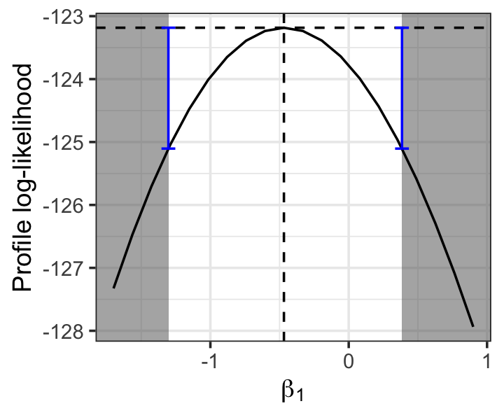
The deviance test’s rejection region is defined by the inequality (Definition 12.10) \[ -2 \log \frac{L(\hat \beta_1)}{\sup_{\beta} L(\beta)} < \chi^2_{1, 1- \alpha}, \] which we may rewrite as \[\begin{align*} \log L(\hat \beta_1) &> \log \sup_\beta L(\beta) - \frac{\chi^2_{1, 1-\alpha}}{2}\\ &> \ell(\hat \beta) - \frac{\chi^2_{1, 1-\alpha}}{2}. \end{align*}\] This region is illustrated in Figure 12.12. In this case, the confidence interval is nearly symmetric because the profile likelihood is, but that need not be the case.
To put the confidence interval on the odds scale, we exponentiate. Often it’s useful to exponentiate all the estimates, and we can do this in one call:
exp(confint(pima_fit)) 2.5 % 97.5 %
(Intercept) 0.004724633 0.3286171
pregnancyYes 0.271584007 1.4697789
bp 1.013722770 1.0710464A 95% confidence interval for the odds ratio associated with having a pregnancy is \([0.272, 1.47]\). This overlaps 1, so we can’t conclusively say whether prior pregnancy is associated with an increase or decrease in odds.
Notice that the point estimate is \(0.626\), so this interval is not symmetric, as expected.
Now that we have two techniques to obtain confidence intervals for \(\beta\), we must ask which to use. In general, the profile likelihood intervals are better: the Wald intervals are only accurate when the sampling distribution of \(\hat \beta\) is symmetric, which may not be the case in small samples, while the profile likelihood intervals work in this case as well as in cases where it is skewed (Pawitan 2001, sec. 2.9). The profile likelihood intervals are hence the better choice, though they are harder to extend to generate intervals for linear combinations \(a\T \beta\), as this would require a multidimensional profile likelihood function.
12.6.3 Deviance tests
For an equivalent of the \(F\) test to compare nested models (Section 11.3), we can use the difference in deviance.
Theorem 12.4 (Deviance test) Consider a full model and a reduced model, where the reduced model is formed by constraining some of the parameters of the full model (e.g. by setting them to zero). The statistic \[ \dev_\text{reduced} - \dev_\text{full} \convd \chi^2_q \] where \(q\) is the difference in the degrees of freedom (number of free parameters) between the two models, and the convergence is as \(n \to \infty\).
Proof. We can write \[\begin{align*} \dev_\text{reduced} - \dev_\text{full} &= 2 \ell_\text{sat} - 2 \ell(\hat \beta_\text{reduced}) - (2 \ell_\text{sat} - 2 \ell(\hat \beta_\text{full})) \\ &= 2 \left(\ell(\hat \beta_\text{full}) - \ell(\hat \beta_\text{reduced})\right) \\ &= - 2\left(\ell(\hat \beta_\text{reduced}) - \ell(\hat \beta_\text{full})\right) \\ &= - 2 \log \left(\frac{L(\hat \beta_\text{reduced})}{L(\hat \beta_\text{full})}\right), \end{align*}\] where \(L(\beta)\) is the likelihood function. This is now a likelihood ratio test as described in Section 11.3.2, and the standard results for the asymptotic distribution of likelihood ratio tests can be applied.
Example 12.13 (Deviance tests in R) Let’s again consider the diabetes data from Example 12.5. Besides blood pressure and prior pregnancy status, the data also contains the age of each patient and their blood glucose measurement. Let’s test the two models against each other.
pima_larger_fit <- glm(type ~ pregnancy + bp + age + glu,
                       data = Pima.tr, family = binomial())

anova(pima_fit, pima_larger_fit, test = "Chisq")
Analysis of Deviance Table
Model 1: type ~ pregnancy + bp
Model 2: type ~ pregnancy + bp + age + glu
Resid. Df Resid. Dev Df Deviance Pr(>Chi)
1 197 246.37
2 195 194.34 2 52.031 5.032e-12 ***
---
Signif. codes: 0 '***' 0.001 '**' 0.01 '*' 0.05 '.' 0.1 ' ' 1As you can see, the anova.glm() method for anova() can automatically calculate the deviances and conduct the test; the test = "Chisq" option (which is equivalent to test = "LRT") specifies the deviance test defined in Theorem 12.4.
Exercise 12.2 (Interpreting a deviance test) Write down the null hypothesis for the test shown in Example 12.13, and give the test’s result in APA format.
12.7 Reporting results
In published work using logistic regression, such as papers in medical, psychological, or biological journals, results are typically reported in a table giving the model terms and their odds ratios. Results are explained in the text using odds ratios, their confidence intervals, and any relevant tests. It’s rare to see log-odds reported directly, since log-odds are hard to interpret on their own; while odds ratios must be interpreted carefully, they at least have a more direct interpretation, and readers will be used to them.
Example 12.14 (Reporting a logistic fit) Suppose the model from Example 12.5 were being reported in a paper. In the Methods section, after a detailed description of the data and how it was obtained, we might expect a sentence like this:
To examine the relationship between pregnancy, blood pressure, and diabetes in Pima women, we fit a logistic regression model to predict diabetes status using diastolic blood pressure and prior pregnancy status.
There might then be a few sentences discussing model diagnostics, as discussed in Section 12.5, to justify the choice of a logistic regression model with blood pressure linearly associated with the log-odds of diabetes. It is not necessary to give a model formula or mathematical equation, since in applied journals, most readers will be familiar with logistic regression, and the description above is clear.
In the Results section, a table would give the model fit. The code below produces a common style of table using the gtsummary package. Notice that this table gives odds ratios, not log odds (because of the exponentiate = TRUE argument), and it includes confidence intervals and \(p\) values. Odds ratios and confidence intervals are the most useful for interpretation. (The additional cols_align_decimal() step is to align numbers at their decimal point, making their magnitude easier to judge compared to others in the same column.)
library(gtsummary)
library(gt)

tbl_regression(pima_fit, intercept = TRUE, exponentiate = TRUE) |>
  as_gt() |>
cols_align_decimal(c(estimate, p.value))| Characteristic | OR | 95% CI | p-value |
|---|---|---|---|
| (Intercept) | 0.04 | 0.00, 0.33 | 0.003 |
| pregnancy | |||
| No | — | — | |
| Yes | 0.63 | 0.27, 1.47 | 0.3 |
| bp | 1.04 | 1.01, 1.07 | 0.004 |
| Abbreviations: CI = Confidence Interval, OR = Odds Ratio | |||
In the text of the Results section, we might expect sentences such as:
Table 12.3 gives the results of the logistic regression fit. Women with prior pregnancies were less likely to have diabetes (\(\text{OR} = 0.626\), 95% CI [0.27, 1.5]), but this result was not statistically significant (\(z = -1.1\), \(p = 0.27\)). A larger sample may be necessary to determine if a relationship exists in the population.
In fields where logistic regression analyses are common, odds ratios are typically presented directly, without an interpretation in terms of the change in odds as covariates change. This is particularly the case when covariates are binary, such as the presence or absence of a medical condition.
Example 12.15 (COVID comorbidities) Harrison et al. (2024) used electronic medical records and logistic regression to study which medical conditions were associated with a higher risk of death from COVID-19. Their structured abstract (see Section 24.1.1) is very direct:
Background. At the beginning of June 2020, there were nearly 7 million reported cases of coronavirus disease 2019 (COVID-19) worldwide and over 400,000 deaths in people with COVID-19. The objective of this study was to determine associations between comorbidities listed in the Charlson comorbidity index and mortality among patients in the United States with COVID-19.
Methods and findings. A retrospective cohort study of adults with COVID-19 from 24 healthcare organizations in the US was conducted. The study included adults aged 18–90 years with COVID-19 coded in their electronic medical records between January 20, 2020, and May 26, 2020. Results were also stratified by age groups (<50 years, 50–69 years, or 70–90 years). A total of 31,461 patients were included. Median age was 50 years (interquartile range [IQR], 35–63) and 54.5% (n = 17,155) were female. The most common comorbidities listed in the Charlson comorbidity index were chronic pulmonary disease (17.5%, n = 5,513) and diabetes mellitus (15.0%, n = 4,710). Multivariate logistic regression analyses showed older age (odds ratio [OR] per year 1.06; 95% confidence interval [CI] 1.06–1.07; \(p < 0.001\)), male sex (OR 1.75; 95% CI 1.55–1.98; \(p < 0.001\)), being black or African American compared to white (OR 1.50; 95% CI 1.31–1.71; \(p < 0.001\)), myocardial infarction (OR 1.97; 95% CI 1.64–2.35; \(p < 0.001\)), congestive heart failure (OR 1.42; 95% CI 1.21–1.67; \(p < 0.001\)), dementia (OR 1.29; 95% CI 1.07–1.56; \(p = 0.008\)), chronic pulmonary disease (OR 1.24; 95% CI 1.08–1.43; \(p = 0.003\)), mild liver disease (OR 1.26; 95% CI 1.00–1.59; \(p = 0.046\)), moderate/severe liver disease (OR 2.62; 95% CI 1.53–4.47; \(p < 0.001\)), renal disease (OR 2.13; 95% CI 1.84–2.46; \(p < 0.001\)), and metastatic solid tumor (OR 1.70; 95% CI 1.19–2.43; \(p = 0.004\)) were associated with higher odds of mortality with COVID-19. Older age, male sex, and being black or African American (compared to being white) remained significantly associated with higher odds of death in age-stratified analyses. There were differences in which comorbidities were significantly associated with mortality between age groups. Limitations include that the data were collected from the healthcare organization electronic medical record databases and some comorbidities may be underreported and ethnicity was unknown for 24% of participants. Deaths during an inpatient or outpatient visit at the participating healthcare organizations were recorded; however, deaths occurring outside of the hospital setting are not well captured.
Conclusions. Identifying patient characteristics and conditions associated with mortality with COVID-19 is important for hypothesis generating for clinical trials and to develop targeted intervention strategies.
Notice that each comorbidity is listed with the odds ratio, its 95% confidence interval, and the \(p\) value for the Wald test that \(\beta = 0\). (Evidently the journal does not require the \(z\) scores to be presented, as they are not listed in the Results section either.) The abstract also briefly states the composition of the sample (adults age 18–90 treated by 24 healthcare organizations in the US in a specific time period, with brief summaries of age, gender, and comorbidities). But as it is written for a medical audience familiar with the use of logistic regression for analyses like these, it does not try to explain how each coefficient means the odds are multiplied by a certain amount—the reader is expected to understand this.
Exercises
Exercise 12.3 (Algebra with the logit function) Show that \(\ilogit(\logit(p)) = p\), and that the different ways to write the model in Definition 12.1 are equivalent.
Exercise 12.4 (Algebra with the logistic likelihood) Derive the expression for the log-likelihood function \(\ell(\beta)\) given in Section 12.2 from the definition of the likelihood function \(L(\beta)\) and the form of the logistic regression model.
Exercise 12.5 (Perfect separation) Suppose we have one predictor \(x \in \R\), where \[ Y = \begin{cases} 1 & \text{if $x > x_0$} \\ 0 & \text{if $x \leq x_0$}, \end{cases} \] and we have \(n > 2\) samples from this population. Consider fitting a logistic regression model such that \[ \Pr(Y = 1 \mid X = x) = \ilogit(\beta_0 + \beta_1 x). \] What would the maximum likelihood estimate of \(\beta_1\) be? A formal proof is not required; a heuristic or graphical argument is fine.
This situation can sometimes occur in real data with multiple predictors, when there is a plane in \(\R^p\) such that observations with \(X\) on one side have \(Y = 1\) and those on the other side have \(Y = 0\).
Exercise 12.6 (EDA in logistic regression) The CMU S&DS Data Repository includes a dataset on bacterial and viral meningitis. The task is to determine whether a patient’s meningitis is caused by a bacterial or a viral infection using blood and cerebrospinal fluid (CSF) test results, so appropriate treatment can be started immediately.
Download meningitis.csv and review the repository’s description of the dataset and variables. Use empirical link plots (Example 12.7) to examine the relationship between the following variables and the type of meningitis (the abm variable):
- CSF glucose level (
gl) - CSF protein level (
pr) - CSF leukocyte count (
whites) - Percent of polymorphonuclear leukocytes (PMNs) in CSF (
polys)
For each, examine the relationship and judge whether it would be helpful to transform the predictor. Then judge whether the relationship between the predictor and the log-odds is linear, or whether a nonlinear logistic model would be more appropriate. A formal test is not necessary; base your judgments on the plots.
Note the variables have many missing values, which you can remove; the na.rm argument to mean() and empirical_link() will be helpful.
Exercise 12.7 (Interpreting coefficients) Using the coefficients in Table 12.1, calculate the following by doing the math by hand or with R (by adding the relevant coefficients, not by using predict() or similar):
- The change in log-odds of diabetes and the odds ratio associated with a blood pressure increase of 10 mm Hg.
- The predicted log-odds, odds, and probability of diabetes for a Pima woman with a prior pregnancy and a blood pressure of 70 mm Hg.
- The difference in log-odds, the odds ratio, and the change in probability of diabetes between Pima women with and without a prior pregnancy, among those with a blood pressure of 70 mm Hg.
Exercise 12.8 (Interpreting coefficients with interactions) Let’s consider an example with two factor variables and an interaction, as interactions can be more difficult to interpret. One definition classifies people as having high blood pressure if their diastolic blood pressure is over 85 mm Hg and their systolic blood pressure is over 130 mm Hg. Let’s create a binary variable for high blood pressure in the Pima data of Example 12.5, and interact it with the pregnancy variable.
Pima.tr$highbp <- ifelse(Pima.tr$bp >= 85, "High", "Normal")

pima_interact <- glm(type ~ pregnancy * highbp, data = Pima.tr,
                     family = binomial())
(Yes, as we discussed in Section 9.2.4, dichotomization throws away information; but often doctors will demand classification of things like high blood pressure because a dichotomous rule is used clinically, and in any case we’re using this merely to create an example of an interaction.)
The estimated coefficients are shown in Table 12.4.
| Term | Estimate | SE | \(\exp(\text{Estimate})\) | z | p |
|---|---|---|---|---|---|
| (Intercept) | 0.000 | 0.816 | 1.000 | 0.000 | 1.000 |
| pregnancyYes | -0.134 | 0.967 | 0.875 | -0.138 | 0.890 |
| highbpNormal | -0.368 | 0.925 | 0.692 | -0.398 | 0.691 |
| pregnancyYes:highbpNormal | -0.289 | 1.073 | 0.749 | -0.269 | 0.788 |
- For a Pima woman with no prior pregnancy, what is the odds ratio for high blood pressure? (That is, the odds of diabetes for women with high blood pressure, divided by the odds for those with normal blood pressure.)
- For a Pima woman with at least one prior pregnancy, what is the odds ratio for high blood pressure?
- For a Pima woman with normal blood pressure, what is the odds ratio for having a prior pregnancy?
- Why is the estimate for the intercept exactly 0? What does this imply about the number of women with and without diabetes, among those women in the sample with no prior pregnancies and high blood pressure?
- Conduct a Wald test (Theorem 12.3) for the null hypothesis that pregnant women with normal blood pressure have the same risk of diabetes as not-pregnant women with high blood pressure. Do this manually, using the coefficients (from
coef()) and their estimated covariances (fromvcov()).
Exercise 12.9 (An interaction paradox) Consider the following hypothetical situation, as described by Rohrer and Arslan (2021):
A large company is testing a mentoring program with the hope of increasing employee retention. For this purpose, 10% of employees have been randomly assigned to participate in the program, and the company plans to evaluate its effects on quitting 1 year later. But then a global pandemic forces a change of plan, and because of distancing measures, only half of the employees can work on site, with the other half working remotely. The decision who still works on site has been randomized. All the while, the mentoring program is continued through video conferencing.
Once the time has come for the evaluation of the mentoring program, there are now two questions that can be evaluated: Did the mentoring program reduce quitting? And did it do so equally for on-site and remote workers—in other words, was there an interaction between the mentoring program and work location?
One could use logistic regression to analyze this data, and a hypothetical fit is shown in Table 12.5.
| Variable | Estimate |
|---|---|
| Intercept | -3.06 |
| Mentoring | -1.46 |
| Working on site | 2.90 |
| Mentoring × Working on site | 0.87 |
Using the table, answer the following questions.
- Calculate the log-odds of quitting for remote workers, both for those who received mentoring and those who did not. Calculate the difference. This is the treatment effect for remote workers.
- Repeat the calculation for those who worked on site. Which group had a larger treatment effect on the log-odds scale?
- Now calculate the probability of quitting for remote workers, both for those who received mentoring and those who did not. Calculate the difference, which is the change in probability of quitting from the treatment.
- Finally, repeat this calculation for those who worked on site. Which group had a larger treatment effect on the probability scale? Explain how this could be possible.
This problem illustrates that one must be careful interpreting interactions in logistic regression, and always convert to the appropriate scale (log-odds, odds, or probability) to make the right comparison.
Exercise 12.10 (Misspecified logistic regression) Consider a population where
logit_quad_pop <- population(
  x1 = predictor(rnorm, mean = 0, sd = 10),
  x2 = predictor(runif, min = -5, max = 5),
  y = response(0.7 + 0.2 * x1 - 0.4 * x2**2,
               family = binomial(link = "logit"))
)
Take a sample of \(n = 500\) observations from this population and fit a logistic regression model that only includes linear terms, no quadratics or other polynomial terms.
- Construct the partial residual plots using the
partial_residuals()function from the regressinator, adding a smoothing line withgeom_smooth()(see Example 9.3 for an example in linear models). Show the partial residual plots and comment on what you see. Can you detect the misspecification? - Plot the deviance residuals against each predictor. (The
augment()function from broom defaults to producing deviance residuals for GLMs.) Comment on the differences between these and the partial residual plots. Why does the slope of the trend in the plot for \(X_1\) look so different? - Finally, plot the randomized quantile residuals using
augment_quantile()or its companionaugment_quantile_longer(). Compare these to the partial and deviance residuals.
Exercise 12.11 (Interpreting calibration plots) In Exercise 12.10, you produced diagnostic plots for a misspecified logistic fit. Produce a calibration plot for that fit and comment on its shape. Can you tell the model is misspecified from its calibration?
Exercise 12.12 (Weisberg (2014), problem 12.3) Sometimes, dairy cows lie down and don’t stand up. These are called “downer cows”. A cow might become a downer because of some kind of illness or trauma; and unfortunately, cows are not able to withstand lying down for extended periods, because of the high pressure on their legs and thighs that eventually causes extensive damage. Untreated downer cows may die, or sometimes are euthanized if treatment is not possible. For dairy farmers, it is hence important to notice downers cows, and to understand why they are downers so they can be treated appropriately.
The alr4 package contains the data frame Downer with data from blood samples of 435 downer cows in New Zealand from 1983–1984. See help(Downer) for a full list of variables and the original source of the data. The outcome variable is a factor with levels died and survived, indicating whether the cow survived. Some variables are missing for some cows, because the data comes from veterinary records, and veterinarians may not have ordered all tests for all cows.
Make a contingency table of
outcomeversusmyopathyand comment on what it implies about the association between myopathy and outcome. To support your comment, calculate the survival rate among cows with and without myopathy.A contingency table is a table that shows all combinations of two discrete variables, and the count of observations with each combination. For example, one cell might represent cows with myopathy present who died, and would contain the count of these cows. In this case, your table will be \(2 \times 2\) and contain four numbers. The
xtabs()function may be useful.Fit a logistic regression predicting outcome from myopathy. For each coefficient estimate, write a sentence in APA format giving the coefficient, its meaning, and a 95% confidence interval. Give the odds ratio for myopathy and a 95% confidence interval for it.
Using
predict(), obtain the predicted probability of survival for cows with and without myopathy, and compare these to the fractions you found in part 1. Give 95% confidence intervals for these predicted probabilities.Consider also using the
ureapredictor, which reports the serum urea concentration (mmol/L). Fit a model with myopathy and urea as predictors. Conduct a deviance test to determine whether an interaction term should be included. Report your deviance test result in APA format, and give an effect plot for the chosen model.
Exercise 12.13 (Weisberg (2014), problem 12.2) The alr4 package contains the data frame Rateprof of data from RateMyProfessors, a popular website for student ratings of professors. The data covers 364 instructors at one Midwestern school who had at least 10 ratings over several years, and includes both student ratings and features of the instructor. Each row gives results for one instructor. See help(Rateprof) for a full description of the variables and the source.
Let’s consider the outcome variable pepper, which reports whether the instructor was rated as attractive or not. (This feature was removed from RateMyProfessors in 2018.) We would like to understand how this outcome is related to the instructor’s gender, the discipline they work in, and average student ratings of the quality and easiness of their courses. (These are the predictors gender, discipline, quality, and easiness.)
Conduct an analysis and summarize your results. Structure this as a miniature report: start with a few well-chosen plots or tables as exploratory data analysis, choose an appropriate model, produce relevant diagnostics, and summarize your results. Each part should only be one to two paragraphs; extensive justification and analysis is not required, but you do need to be clear about your methods and the results.
Write your mini-report as though it is for the school’s Vice Provost for Faculty, who has assembled several committees to study student ratings and whether they are appropriate to use in promotion decisions. One committee is studying whether quality ratings could be biased by gender or discipline; your committee is studying whether the pepper ratings simply perpetuate harmful biases against certain groups of instructors.
Exercise 12.14 (Sugary drinks) TODO https://cmustatistics.github.io/data-repository/psychology/sugary-drinks.html
Exercise 12.15 (Power to detect a difference) Consider a medical trial where the outcome is death (\(Y = 1\)) or survival (\(Y = 0\)), and the predictor is a binary indicator of the treatment (\(X = 1\) for the treatment group, \(X = 0\) for the control group). The true population relationship is \[ \Pr(Y = 1 \mid X = x) = \begin{cases} 0.2 & \text{if $x = 1$} \\ 0.1 & \text{if $x = 0$}. \end{cases} \]
Convert these probabilities to log-odds, and write the population relationship in the form of a logistic regression where \[ \logit(\Pr(Y = 1 \mid X = x)) = \beta_0 + \beta_1 x. \] Calculate the values of \(\beta_0\) and \(\beta_1\).
Use the regressinator to define the population using these covariates. Define your population so that 50% of people are in the control group and 50% are in the treatment group. Show the code you used to define the population.
Hint: Review Example 12.1 to see how to define a binary outcome in the regressinator, and use
rbinom()withsize = 1to define the predictor distribution by usingpredictor(rbinom, size = 1, prob = 0.5).Consider testing \(H_0: \beta_1 = 0\) using a Wald test. (This is the test R conducts and prints out in
summary(), or when you usetidy()to get the estimates from a fit.) This null hypothesis is false, so with perfect power we would reject it 100% of the time.Conduct 1000 simulations, each with \(n = 50\), and use the fraction of those that reject the null hypothesis to estimate the power. Also, what is expected number of deaths in each group given the sample size and the probability of death? (You can calculate this from how we defined the population above, and the expected fraction of patients in the treatment and control groups.) Is the power surprising given the expected number?
Hint: Refer back to Example 11.7 for an example of a power simulation using
sampling_distribution(). Here a loop is not necessary, since we are only using one value of \(n\) and \(\beta_1\) is fixed.Repeat the simulation procedure for multiple values of \(n\), from 100 to 500 in increments of 50 (i.e. \(n = \{100, 150, 200, \dots, 500\}\)). Plot the power against sample size, and report the smallest sample size with power of at least 80%.
(You can use fewer than 1000 simulations per \(n\) if the simulation takes too long to be practical.)
This exercise demonstrates that even when the relative risk is large—the treatment group has twice the risk of the control group!—the power can be low, and a surprisingly large sample size can be required. Partly this is because the probability is low in both groups; it would be easier to detect a difference when, say, the probability is 0.6 and 0.3, even though the relative risk is identical. It’s important to keep power in mind when analyzing real data, particularly for rare effects.
Exercise 12.16 (Interpreting factors in logistic regression) The file logistic-interpret.csv contains a simple dataset with two binary predictors, x1 and x2, and a binary response, y.
Load the data into R. Leave it as-is—don’t convert any values to factors or recode them yet.
Fit a logistic regression with the model formula
y ~ x1 + x2. Look at the intercept coefficient and interpret it: The intercept means the probability of [blank] is [blank] for cases where [blank].Now fit a model with the formula
y ~ x1 + x2 - 1. (See Section 6.2 on formula syntax.) Examine the model summary. Explain what removing the intercept has done: The model assumes the probability of [blank] is [blank] for cases where [blank].Next, convert
x1andx2to factor variables, converting 0 toFand 1 toT. R treats the first level as the baseline, so ensure 0/Fis the first level of each.Repeat the model from part 1. Your result should be identical. Interpret the coefficient R calls
x1Tas an odds ratio. What precisely does the odds ratio mean?Suppose we changed the ordering of the levels of
x1, soTis the baseline (but it’s still 0 =Fand 1 =T). R will print a coefficient labeledx1Finstead ofx1T.Without changing the ordering or fitting the model, say what the odds ratio for
x1Fwill be, and interpret it as in part 3.Finally, fit a model with the formula
y ~ x1 + x2 - 1, again using the data wherex1andx2have been converted to factor variables. Notice that R fits three coefficients: two forx1and only one forx2. With no intercept, R knows it can’t collapse the base level of both factors into the intercept.Get the predicted probabilities for each case from this model and compare them to the model in part 3. Are the models different?
Examine the coefficients. Interpret the
x1Fandx1Tcoefficients. Are they odds or odds ratios? What cases do they describe?Hint: If you’re not sure what R has done, you can also get the model matrix (using
model.matrix()) to see how it encoded the variables, or make predictions (usingpredict()) to see how the predictions correspond to the coefficients.
The point here is that coefficients can represent log-odds or changes in log-odds (odds or odds ratios), and because R automatically codes factors (Section 7.4), the meaning of a coefficient can depend on R’s decisions on what to do with the factors. You must pay attention to interpret coefficients correctly.
“Ham” by contrast with spam, the canned meat-like product.↩︎
This is not strictly true: you could make a model that fits worse than the null model, although you’d have to try. If your model includes the null model as a special case, and you use maximum likelihood, you cannot fit worse than the null model; if you pick the parameters some other way, or devise a model that does not include the null model as a special case, you could perhaps do so.↩︎
In their original paper, Dunn and Smyth (1996) used the standard normal CDF to transform the standardized residuals to be normally distributed, better matching the residuals from linear models. But it is easier to see a uniform distribution by eye than a normal distribution, so later work omits this step.↩︎
And if it did, we likely would not need a complex model that requires diagnostics: simply use the observed fraction of ones as your prediction for that \(x\).↩︎
It may be tempting to use the delta method to get the distribution of the transformation, but remember the confidence intervals may not be symmetric—and they certainly will not be once we exponentiate. The delta method would ignore this.↩︎