21 Mixed and Hierarchical Models

In the linear and generalized linear models so far, the regression parameters ($\beta$) are fixed properties of the population, and our task is to estimate them with as much precision as possible. We then interpret the parameters to make statements about the population. The parameters are fixed, so their effects are known as fixed effects.

But it is possible for the relationship between predictor and response to also depend on random quantities—on properties of the particular random sample we obtain. When this happens, some of the model parameters are random, and so their effects are known as random effects.

We can construct linear and generalized linear models with random effects, known as random effects models or mixed effects models (“mixed” because they contain both fixed and random effects). As we will see, these are useful for modeling many kinds of data with grouped or repeated structure. They can also be thought of as a way of applying penalization, as discussed in Chapter 19, to regression coefficients in a more structured way, and so can give useful estimates even when the parameters are not truly random.

21.1 Motivating examples

Many regression problems involve data that comes from a random sample from a population (or that we at least treat as a random sample). But we are concerned with problems where the effects are random. For instance, if the observations come in groups, perhaps the relationship is different for each group, and perhaps the groups can be seen as samples from a larger population.

Example 21.1 (Small area estimation) A social scientist is constructing a map of poverty across the United States as part of a project to suggest government policies that might help low-income areas. The scientist wants to estimate the average income of individuals in every county in the US, and pays a polling company to conduct a large, representative national survey. Survey respondents indicate their county of residence and their income.

Each observation is one person, but we want to estimate county averages, so it is reasonable to model respondent $i$’s income as \[ \text{income}_i = \alpha_{\text{county}[i]} + e_i, \] where $\text{county}[i]$ represents the index of the county respondent $i$ lives in. As there are about 3,200 counties, $\alpha$ is a vector of about 3,200 values, and their estimates $\hat \alpha$ give us the average income per county. We can treat $\alpha$ as a fixed unknown parameter, making this a simple regression or ANOVA problem; or we can imagine the counties as a sample from the process generating county incomes every year, making them random effects. As we will see, this has some advantages.

This is an example of a small area estimation problem, in which the goal is to make inferences about individual geographic areas from survey or sample data. The data is hierarchical: the units are survey respondents, who are grouped within counties, which are all within the United States.

Example 21.2 (Sleep deprivation) Belenky et al. (2003) conducted an experiment to measure the effect of sleep deprivation on reaction time. A group of 18 experimental subjects spent 14 days in the laboratory. For the first 3 nights, they were required to be in bed for eight hours per night; for the next seven days, they were only allowed three hours per night. Each day, they completed several tests of alertness and reaction time, including one that directly measured how quickly they pressed a button after seeing a visual stimulus. Our data hence includes 10 observations per subject: three days of baseline measurements and seven days of sleep deprivation.

The goal is to measure the effect of sleep deprivation on reaction time, including how reaction time changes as the number of days of deprivation increases. We might model respondent $i$’s reaction time on day $d$ as \[ \text{time}_{id} = \beta_0 + \beta_1 d + e, \] but it is reasonable to expect that each subject had a different reaction time at baseline (0 days) and that each was affected differently by sleep deprivation. If this is not accounted for, the errors $e$ will be dependent between observations of the same subject on different days.

Instead we might allow both the slope and intercept to vary by subject: \[ \text{time}_{id} = \alpha_i + \beta_i d + e. \] As subjects are drawn from a population, here $\alpha$ and $\beta$ are both random effects.

These examples also illustrate a difference in goals between mixed model problems. In Example 21.1, we would like to estimate the individual random effects $\alpha$ for each county. In Example 21.2, the subject-specific slopes and intercepts are not important: the scientific question is whether $\E[\beta_i] = 0$, which determines whether the average person experiences a change in reaction time when sleep-deprived. We will see that mixed models are better suited to answer the latter question, although obtaining individual random effect estimates is still possible.

21.2 Mixed models

From the examples, we see that a mixed model is a regression model much like any other: we have a response variable and one or more predictors, and translate the predictors into regressors to fit the regression. However, in a mixed model we split the predictors into two groups first. The fixed effects are treated just as in ordinary linear models, while the random effects have a separate parameter vector that is random.

As the variance and covariance structure of the random effects will be important, we can separately consider the mean structure of mixed models and the variance structure.

21.2.1 Mean structure

Definition 21.1 (Linear mixed model) A linear mixed model is a linear model written as \[ Y_i = {\underbrace{\beta\T X_i}_{\text{fixed effects}}} + {\underbrace{\gamma\T Z_i}_{\text{random effects}}} + e_i, \] where $\beta \in \R^p$ is a fixed population parameter, $X_i \in \R^p$ is a vector of known covariates, $\gamma \in \R^q$ is a vector of random effects, and $Z_i \in \R^q$ is another vector of known covariates. Crucially, $\gamma$ is a random variable that is assumed to be drawn from a particular distribution. One can also write the model in matrix form as \[ \Y = \beta\T \X + \gamma\T \Z + e. \]

Generally it is assumed that $\E[e] = 0$, $\var(e) = \sigma^2 I$, $\cov(\gamma, e) = 0$, and the distribution of $\gamma$ is a parametric family with mean 0 and known or estimable covariance.

Transforming a particular model into a mixed model simply requires translating its predictors into regressors represented as columns of $X$ and $Z$, just as we did with ordinary linear models in Chapter 7.

Example 21.3 (Random intercepts model) In the small area estimation example (Example 21.1), there is one predictor, county. We will represent this as dummy-coded regressors in $Z$, including a regressor for every county, so none is absorbed in the intercept. The model is \[ \text{income} = \beta_0 + \gamma\T \Z + e, \] $\beta_0$ represents the overall mean across counties (because $\gamma$ has mean zero) and the entries of $\gamma$ give the difference between each county’s mean and the grand mean. The intercept $\beta_0$ is a fixed effect and $\gamma$ is a random effect.

Example 21.4 (Random slopes model) In the sleep deprivation study (Example 21.2), there are two predictors: the number of days of sleep deprivation and the subject. The number of days is a fixed effect, so $X$ contains an intercept column and a column for the number of days; hence $\beta \in \R^2$. Subject is a random effect, and we want this to affect both the intercept and slope, so we will enter multiple regressors in $Z$: an an indicator of subject (and hence a column for every subject) as well as columns for the interaction of subject and days. We can hence partition the random effects part of the model: \[ \gamma\T \Z = \begin{pmatrix} \gamma_1 \\ \vdots \\ \gamma_{18} \\ \gamma_{19} \\ \vdots \\ \gamma_{36} \end{pmatrix}\T \left(\begin{array}{cccc|cccc} 1 & 0 & \cdots & 0 & 0 & 0 & \cdots & 0\\ 1 & 0 & \cdots & 0 & 1 & 0 & \cdots & 0\\ 1 & 0 & \cdots & 0 & 2 & 0 & \cdots & 0 \\ \vdots & \vdots & & \vdots & \vdots & \vdots & & \vdots \\ 0 & 0 & \cdots & 1 & 0 & 0 & \cdots & 7\\ 0 & 0 & \cdots & 1 & 0 & 0 & \cdots & 8\\ 0 & 0 & \cdots & 1 & 0 & 0 & \cdots & 9 \end{array}\right). \] Here the first 18 entries of $\gamma$ correspond to random intercepts for each of the 18 subjects, while the next 18 entries are random interactions for each subject. We then assemble them into the model \[ \text{time} = \beta_0 + \beta_1 d + \gamma\T \Z + e. \] The interaction allows the intercept and slope of the relationship to be random effects, not fixed, with the mean intercept and slope estimated by $\beta_0$ and $\beta_1$. For example, for subject 1 on day $d$, $Z = (1, 0, \dots, 0, d, 0, \dots, 0)\T$, and so the model is \[\begin{align*} \text{time} &= \beta_0 + \beta_1 d + \gamma_1 + \gamma_{19} d + e\\ &= (\beta_0 + \gamma_1) + (\beta_1 + \gamma_{19}) d + e. \end{align*}\]

Thus the average intercept and slope across patients ($\beta_0$ and $\beta_1$) are fixed effects, but the subject-level variation is encoded as random effects (in $\gamma$).

In each case we have written the model to make the mean of the random effects zero, so their mean is estimated as a fixed effect. This is convenient because the software we use for estimation defaults to setting the mean of all random effects to zero.

21.2.2 Variance structure

Besides specifying the mean function, we must specify the covariance structure $\Sigma = \var(\gamma)$. This is not comparable to the variance $\var(\hat \beta)$ for the fixed effect term: that is a property of the estimator $\hat \beta$, and it is silly to refer to $\var(\beta)$ (without the hat) because $\beta$ is a fixed population parameter. For the random effects, $\gamma$ is random, so $\Sigma$ is a population parameter to estimate.

We have several options. We could simply assume $\Sigma$ has a particular value, such as $\Sigma = I$. But that is rarely realistic. We could, at the other extreme, estimate the entire matrix with no assumptions, allowing any variance and covariance between terms in $\gamma$. That may be too flexible, and also is often unrealistic, as we will see in the examples below.

Instead, we usually identify a specific structure for $\Sigma$ and then estimate its component pieces as part of the model-fitting process. Two common structures are given in these examples.

Example 21.5 (Variance in the random intercepts model) Consider the random-intercepts model applied to small area estimation (Example 21.3), where each entry of $\gamma$ is one county’s difference from the overall mean. If counties are drawn independently from a hypothetical county-generating process, we could assume that \[ \var(\gamma) = \sigma_\gamma^2 I. \] If we also assume that $\var(e) = \sigma^2 I$, the model only has three parameters to estimate ($\beta_0$, $\sigma^2$, and $\sigma_\gamma^2$), despite there being over 3,200 individual counties.

However, if the same random effect predictor enters $\Z$ as multiple regressors, it is more reasonable to assume the corresponding entries of $\gamma$ are correlated. This is just as in ordinary linear regression: in a simple linear model $Y = \beta_0 + \beta_1 X + e$, $\cov(\hat \beta_0, \hat \beta_1) \neq 0$ except in special cases. (We can think of $\beta_0$ as being a regressor for $X$ because it is the intercept of the relationship with $X$, just as random intercepts for a grouping variable are intercepts but are regressors for that predictor.)

Example 21.6 (Variance in the random slopes model) In the random slopes model of Example 21.4, it’s not reasonable to say that the entries of $\gamma$ are simply iid with common variance $\sigma_\gamma^2$. The intercept and interaction effects may have different variances, and the effects for subject $i$ are likely correlated with each other, just as the slope and intercept are correlated in an ordinary linear model. A reasonable choice might instead be that $\var(\gamma) = \Sigma$, where \[ \Sigma_{ij} = \begin{cases} \sigma_0^2 & \text{if $i = j$ and $i \leq 18$}\\ \sigma_1^2 & \text{if $i = j$ and $i > 18$}\\ \sigma_{01} & \text{if $|i - j| = 18$}\\ 0 & \text{otherwise.} \end{cases} \] Hence the intercepts have variance $\sigma_0^2$, the interaction slopes have variance $\sigma_1^2$, and the slope and intercept for one subject have correlation $\sigma_{01}$. But by setting the covariance to 0 between subjects, we have assumed the subjects are not correlated with each other. This is logical unless the subjects somehow influence each other’s responses.

The general rule, then, is to evaluate all the random effects terms. Like terms entering from the same predictor—such as all the regressors needed to enter one factor predictor—are modeled with a common variance. Related terms from the same predictor—such as slope and intercept terms—are modeled with a common covariance. Random effects are assumed uncorrelated between unrelated predictors.

21.2.3 Variance components

The effect of the random effects terms in a mixed model is to induce correlation between observations, and to partition the variance of $Y$ into components. We can see this by expanding the variance using Definition 21.1: \[\begin{align*} \var(\Y) &= \var(\beta\T \X + \gamma\T \Z + e) \\ &= \Z \var(\gamma) \Z\T + \var(e) \\ &= \Z \Sigma \Z\T + \sigma^2 I. \end{align*}\] The total variance of the response is hence partly due to the errors $e$ and partly due to the random effects. What this means depends on the structure we assume for $\Sigma$. In simple random intercepts models, for instance, the variance decomposes nicely.

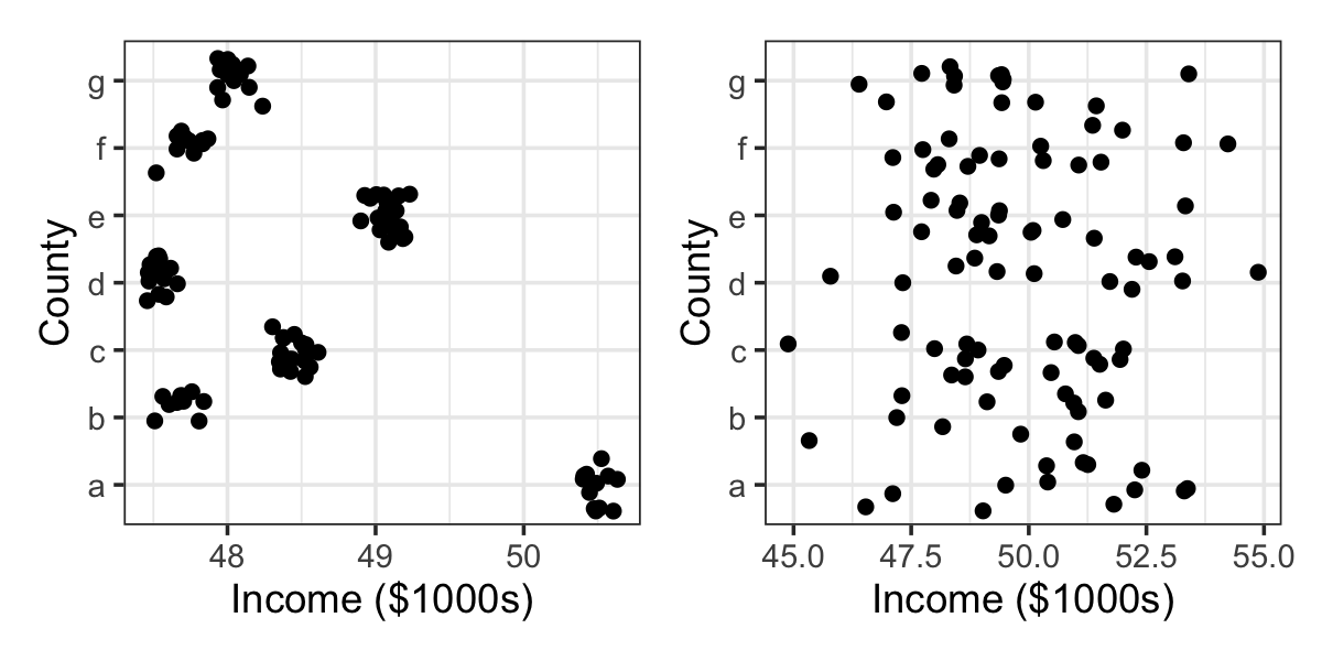
Example 21.7 (Variance components in the random intercepts model) In the random intercepts model for counties, suppose we assume that $\var(\gamma) = \sigma_\gamma^2 I$, as in Example 21.5. There is one predictor per county, so this is an $n \times n$ matrix, and each row of $\Z$ has exactly one 1 and $n - 1$ zeroes (since $\Z$ encodes the county of each observation). Thus, for survey respondent $i$, \[ \var(Y_i) = \var(\gamma\T Z_i + e_i) = \sigma_\gamma^2 + \sigma^2. \] The variance in respondent incomes is then partly due to random noise ($\sigma^2$) and partly due to variation in county means ($\sigma_\gamma^2$). The relative size of $\sigma^2$ and $\sigma_\gamma^2$ determines the structure of the data: if $\sigma_\gamma^2 \gg \sigma^2$, there is a great deal of variation between counties but very little within a county, as shown in the left panel of Figure 21.1. If $\sigma_\gamma^2 \ll \sigma^2$, the reverse is true: the counties are very similar and most variation is individual, as shown in the right panel.

Figure 21.1: *Left:* County-level variation ($\sigma_\gamma^2$) is large relative to subject-level variation ($\sigma^2$). *Center:* County- and subject-level variation are equal. *Right:* Subject-level variation is large relative to county-level variation. Each point is one respondent within a county.

For two respondents $i$ and $j$, where $i \neq j$, the covariance between their responses is \[\begin{align*} \cov(Y_i, Y_j) &= \cov(\gamma\T Z_i + e_i, \gamma\T Z_j + e_j)\\ &= \cov(\gamma\T Z_i, \gamma\T Z_j) + \cov(\gamma\T Z_i, e_j) + \cov(e_i, \gamma\T Z_j) + \cov(e_i, e_j). \end{align*}\] As we said in Definition 21.1, we usually assume that $\cov(\gamma, e) = 0$, so the center two terms are zero. The last term is zero because we typically assume the errors are uncorrelated, as in ordinary linear models. Only the first term matters. When both respondents are in the same county, this is the variance of that component of $\gamma$; when they are not, it is the covariance between the corresponding components. Since we assumed $\var(\gamma)$ is diagonal, \[ \cov(Y_i, Y_j) = \begin{cases} \sigma_\gamma^2 & \text{if in the same county} \\ 0 & \text{otherwise.} \end{cases} \] Thus, marginally, the random effect means the response is correlated for units within the same group: incomes for people in the same county are correlated with each other.

This decomposition is why the variances in mixed-effects models are often referred to as variance components: the total variance of $Y$ is decomposed into components coming from unit-level random error and the fixed effects. We can use the variance components to quantify the decomposition of error by using the intraclass correlation coefficient.

Definition 21.2 (Intraclass correlation coefficient) The intraclass correlation coefficient (ICC) in a simple random intercepts model \[ \Y = \beta_0 + \gamma\T \Z + e, \] where the random effect is a categorical grouping variable, is \[ \operatorname{ICC} = \cor(Y_i, Y_j) \] for two units $i$ and $j$ in the same group.

When $\var(\gamma) = \sigma_\gamma^2 I$ and $\var(e) = \sigma^2$, \[ \operatorname{ICC} = \frac{\sigma_\gamma^2}{\sigma^2 + \sigma_\gamma^2}, \] by definition of the correlation.

The ICC is between 0 and 1. When the ICC is 0, the random effect variance is 0, and all variation is due to the unit-level random error; when the ICC is 1, the unit-level random error variance is 0, and all variation is due to the random effect. In Figure 21.1, the left panel ICC is nearly 1 and the right panel ICC is nearly 0. The ICC is thus a useful summary of the variation in a random effects model, and estimating the variances is hence a key part of the estimation process.

21.2.4 The generative model

Typically, linear mixed models assume normally distributed errors, as in ordinary linear models, and normally distributed random effects. This implies a two-step generative model for the data:

Draw $\gamma \sim \normal(\zerovec, \Sigma)$.
Draw $e \sim \normal(\zerovec, \sigma^2 I)$, and let $\Y = \beta\T \X + \gamma\T \Z e$.

If the random effects are from grouping variables, this is a hierarchical structure: generate the group parameters first, then use these to generate the observations. Thus we often refer to mixed models as hierarchical models.

Example 21.8 (Generating random intercepts) The random intercepts model of Example 21.3, with normal errors and normal random effects, is equivalent to the model where \[\begin{align*} \alpha &\sim \normal(0, \sigma_\gamma^2 I) \\ Y_i &\sim \normal(\beta_0 + \alpha_{\text{county}[i]}, \sigma^2). \end{align*}\] Here $\alpha$ is a vector of county means and $\alpha_{\text{county}[i]}$ is the mean for the county of observation $i$.

TODO some kind of diagram showing overlapping distributions

Example 21.9 (Generating random slopes) The random slopes model of Example 21.4, with normal errors and normal random effects, is equivalent to the model where \[\begin{align*} \begin{pmatrix} \alpha_j \\ \delta_j \end{pmatrix} &\sim \normal\left(\zerovec, \begin{pmatrix} \sigma_0^2 & \sigma_{01} \\ \sigma_{01} & \sigma_1^2 \end{pmatrix} \right) \\ Y_i &\sim \normal\left((\beta_0 + \alpha_{\text{subject}[i]}) + (\beta_1 + \delta_{\text{subject}[i]}) d, \sigma^2 \right). \end{align*}\] Here $\alpha_j$ is the change in intercept for subject $j$, $\delta_j$ is their change in slope, and $\text{subject}[i]$ is the subject associated with observation $i$. The slope and intercept are correlated as described in Example 21.6, making this slightly harder to write. The random effects mean each subject has a different slope and intercept, but as they have mean zero, the average slope and intercept are $\beta_1$ and $\beta_0$, which are fixed population parameters.

Mixed models need not be completely hierarchical, however, if we have multiple random effects coming from multiple overlapping grouping variables.

21.2.5 Choosing between fixed and random effects

To fit a mixed model, we have to decide which predictors to include as fixed effects (in $\X$) and which to include as random effects (in $\Z$). How should we decide?

Because the random effect parameter $\gamma$ is modeled as a random variable, we only obtain estimates of its mean and variance. (It is possible to obtain post-hoc estimates of $\gamma$ itself, as we’ll see in Section 21.3.3, but those do not permit easy inference.) Random effects thus aren’t suitable for effects of primary interest, such as treatment variables. Instead, they’re best suited for effects that vary between subjects or units, where the interest is in the average value or the variance, not in the individual unit effects.

For example:

In a medical experiment, we may have multiple measurements from the same subject before and after a treatment. These are known as repeated measures. We expect variation between subjects and correlation between measurements of the same subjects. Adding a subject random effect can model both of these, while keeping a fixed effect to estimate the treatment effect.
In an educational experiment, we might assign different course sections to use different teaching strategies, then record the grades of students in each section. The observations are students, but there is undoubtedly correlation between students in each section, and variation from section to section based on the instructor, class time, and other factors. A section random effect could account for this.
In a policy study, we might pull Medicaid records from multiple states to study usage of healthcare by its recipients. Medicaid is an insurance program administered by each state, so its details may vary from state to state. We may thus expect there to be state-level effects that shift the response for all recipients within each state. If we are interested in recipient-level information and not in the state-by-state differences, a state random effect may be appropriate.

It is a little unsatisfying that the “right” model for the data depends on our intention, not just the data-generating process. As a result, there is a confusing variety of advice on whether to treat particular effects as fixed or random. Gelman (2005), section 6, lists five different definitions of the distinction between fixed and random effects, several of which are mutually contradictory. The conceptually simplest answer is to switch to Bayesian hierarchical models (Section 21.8), in which every parameter is random and we infer posterior distributions for them all. In the frequentist mixed model setting, a simple rule is to use random effects whenever there is a grouping variable that affects intercepts and slopes, and not to be afraid of post-hoc estimates of $\gamma$.

TODO add advice somewhere on the right structure of mixed models, e.g., allowing heterogeneity in slopes when you do for intercepts https://doi.org/10.1016/j.jml.2012.11.001

21.3 Estimating mixed models

Estimating the parameters of a mixed model is more complicated than in ordinary linear regression. Only in simple cases can we reduce the problem to simple sums of squares; more complex covariance structure, such as in Example 21.4, means standard least-squares geometry does not apply. We have to estimate multiple variance parameters. The typical approach is to assume parametric distributions for the random effects $\gamma$ and the errors $e$ so that we can use maximum likelihood.

21.3.1 The likelihood

For ordinary regression, the most common approach is to write the mixed model of Definition 21.1 with normally distributed errors and random effects: \[\begin{align*} \Y \mid \gamma &\sim \normal(\beta\T \X + \gamma\T \Z, \sigma^2 I)\\ \gamma &\sim \normal(\zerovec, \Sigma), \end{align*}\] where $\Sigma$ is a covariance matrix giving the covariance of the random effects. We can then marginalize to obtain the marginal model for $\Y$.

Theorem 21.1 (The normal mixed model) The mixed model of Definition 21.1, with normally distributed errors and normally distributed random effects, can be written marginally as \[ \Y \sim \normal(\beta\T \X, \sigma^2 I + \Z \Sigma \Z\T). \]

Proof. See Exercise 21.2.

Hence the likelihood of $\Y$ can be written using the normal density in terms of $\beta$, $\sigma^2$, and $\Sigma$. Notice that $\gamma$ does not appear in the marginal likelihood, so we cannot maximize the likelihood with respect to it! Its variance matrix $\Sigma$ has $q^2$ entries, making it difficult to estimate in general, but when it is structured there may only be a few parameters to estimate (as in Example 21.5 and Example 21.6).

21.3.2 Maximum likelihood and optimization

In principle, maximum likelihood estimation is straightforward and just requires us to maximize with respect to $\beta$, $\sigma^2$, and $\Sigma$. In practice, however, maximum likelihood estimation is difficult here. The $q \times q$ covariance matrix $\Sigma$ has $q^2$ parameters to estimate, and it is constrained, since covariance matrices must be positive definite; such a constraint is difficult to work with. If we assume a specific structure for $\Sigma$, Example 21.5 and Example 21.6, the optimization is easier.

But suppose, for instance, we let $\var(\gamma) = \sigma_\gamma^2 I$. It is entirely possible for the MLE to be $\hat \sigma_\gamma^2 = 0$, which is on the boundary of the space, and the gradient of the likelihood may not be zero. That is, the likelihood may improve as we shrink $\hat \sigma_\gamma^2$ toward zero, without ever reaching a stationary point. Thus, simply taking derivatives and setting them to zero does not suffice to find the MLE. We will likely need a numerical maximizer, and those frequently do not like finding solutions that are exactly on the boundary.

But the problem is not just optimization: The maximum likelihood estimates of the variance are biased. This is true even in ordinary linear regression: Theorem 5.2 showed that the unbiased estimator of $\sigma^2 = \var(e)$ in a simple linear regression model is \[ S^2 = \frac{\RSS(\hat \beta)}{n - p}, \] where $p$ is the number of regressors and $\RSS(\hat \beta)$ is the residual sum of squares. But the maximum likelihood estimate is \[ \hat \sigma^2_\text{MLE} = \frac{\RSS(\hat \beta)}{n}. \]

This is a critical problem in many mixed model applications, as we often interpret the variance components and intraclass correlation (Definition 21.2). This is a natural way to measure the “size” of the random effects, but if the variance estimates are all biased, variance component estimates will all be biased.

Worse, in some mixed model settings the number of parameters grows with $n$. For example, if we have a fixed effect for a factor variable, and the number of levels of that factor grows with $n$, the number of fixed effect parameters will grow with $n$. In this case, the MLE is inconsistent: as $n \to \infty$, the MLE does not converge to the true parameter values. This is called the Neyman–Scott problem.

One solution is restricted maximum likelihood estimation, known as REML. This amounts to finding clever ways to rewrite the likelihood so we can estimate the random effects variances alone, without estimating the fixed effects, and then using these to estimate the fixed effects. The details are out of the scope of this course; see Bates et al. (2015), section 3, or Christensen (2020), section 12.6.

21.3.3 Obtaining random effects estimates

Maximizing the (restricted) likelihood of a mixed effects model gives us values for $\hat \beta$, $\hat \sigma^2$, and $\hat \Sigma$. But $\gamma$ is a random variable, not a parameter, so we do not get estimates of the random effects! Instead, we can treat this as a prediction problem. Just as we build a predictor $\hat Y$ for the random quantity $Y$ in a regression, we can build a predictor $\hat \gamma$ for the random quantity $\gamma$ here.

In regression, the approach is to estimate $\E[Y \mid X = x]$, so here we will estimate the conditional mean $\E[\gamma \mid \Y]$.

Theorem 21.2 (BLUP for random effects) The best linear unbiased predictor (BLUP) of $\gamma$ in a mixed-effects model is \[ \E[\gamma \mid \Y] = \Sigma \Z\T \var(\Y)^{-1} (\Y - \X \beta), \] which may be estimated by \[ \hat \gamma = \hat \Sigma \Z\T \widehat{\var}(\Y)^{-1} (\Y - \X \hat \beta). \]

TODO define what BLUP is, give more reasoning

Proof. See Harville (1976).

We also justify the BLUP using a (vaguely) Bayesian setup for $\gamma$. We have a prior distribution $p(\gamma)$ specified in our mixed model ($\normal(\zerovec, \Sigma)$) and we have a likelihood $p(\Y \mid \gamma)$, treating all parameters as fixed. We can use Bayes’ theorem to obtain the posterior $p(\gamma \mid \Y)$. Because the likelihood and prior are both normal, the posterior is also normal, making it straightforward to derive the posterior mean. The result is the BLUP. TODO derive or make this an exercise

This is known as an “empirical Bayes” procedure. In a fully Bayesian procedure, we would specify priors for all parameters (including the parameters defining $\Sigma$) and obtain the posterior distribution of $\gamma$. In this procedure, we fixed the parameters at their MLEs, even those in the prior distribution of $\gamma$. Since our prior depends on the data, it is “empirical”, hence empirical Bayes.

However you justify it, the BLUP can be used to make predictions of $\gamma$, though of course we still cannot conduct hypothesis tests for $\gamma$ because it is not a population parameter.

21.4 Inference

Conducting inference for mixed models is somewhat more complicated than in ordinary linear models, for the same reason that maximizing the likelihood can be difficult: MLEs for key parameters are biased, and the MLE may be on the boundary of the parameter space. (One of the regularity conditions of Theorem 12.1, which gives the asymptotic distribution of MLEs, is that the parameter not be on the boundary of the parameter space.)

21.4.1 Hypothesis tests

For the fixed effect parameters $\beta$, it is difficult to derive the null distribution of $\hat \beta$ in general, because it depends on $\X$, $\Z$, and $\var(\gamma)$. A common approach is to condition on the estimated variance $\hat \Sigma = \widehat{\var}(\gamma)$; if this is treated as fixed, we can derive least-squares estimates for $\hat \beta$ and its variance, following standard least-squares theory (Pinheiro and Bates 2000, 66). These estimates, however, do not account for uncertainty in $\hat \Sigma$. One can derive Wald tests or $t$ tests based on them, but the null distributions will not be correct, leading to biased $p$ values.

It is not possible to test null hypotheses involving $\gamma$ itself, because $\gamma$ is a random variable, not a parameter. We can only test its variance parameter $\var(\gamma) = \Sigma$, which can be useful if we want to test the presence of a random effect: as we assume $\gamma \sim \normal(\zerovec, \Sigma)$, if $\Sigma$ is the zero matrix, the random effects are all zero and the random effect term can be omitted.

One reasonable approach is a likelihood ratio test (Theorem 11.2). However—and you should get used to “however” appearing frequently in inference for mixed models—the asymptotic distribution of the likelihood ratio statistic depends on certain regularity conditions, and again, one of those conditions is that the parameter not be on the boundary of the parameter space. And the variances being zero is certainly on the boundary. Consequently, even as $n \to \infty$, the likelihood ratio statistic will not approach the $\chi^2$ distribution given by Theorem 11.2. In some cases the null distribution can be calculated (Crainiceanu and Ruppert 2004); in most cases we just accept the usual likelihood ratio test as an approximation.

21.4.2 Confidence intervals

There are, again, several approaches to produce confidence intervals in mixed models. For fixed effects, we can use the approximate Wald confidence intervals based on conditioning on $\hat \Sigma$. But for both fixed and random effects parameters, a better alternative is profile likelihood confidence intervals (Definition 12.10). As long as the parameter values are not at or near the boundary (i.e., as long as a variance is not estimated to be zero), these can be computed and used.

21.4.3 Making predictions

Making predictions from a fitted mixed effects model is not trivial. In principle, the maximum likelihood fit did not estimate the random effects vector $\gamma$, only its mean and variance. Thus we cannot simply plug in new covariate vectors $X$ and $Z$ and obtain \[ \hat Y = \hat \beta\T X + \hat \gamma\T Z. \] Instead, we have two choices:

Marginal predictions: Predict $\E[Y \mid X = x]$, marginalizing over $\gamma$. This predicts the average across all levels of the random effects.
Conditional predictions: Predict $\E[Y \mid X = x, Z = z]$ for a specific random effect vector $z$. This requires an estimate $\hat \gamma$, such as the BLUP (Theorem 21.2).

Marginal predictions are easy but do not permit us to make predictions for individual units with particular random effect vectors. For example, if we use random effects to account for patient-level variability in a medical study, the marginal predictions will be for the average patient, not for any individual patient.

Conditional predictions can only be produced for random effect vectors already observed in the data. For example, if we use a patient-level random effect in a medical study, $\gamma$ gives the patient random effects, so a post-hoc estimate of $\hat \gamma$ can be used to make predictions for the observed patients. But if we then enroll a new patient and want to make a prediction for them, we cannot: adding one new level to the patient factor variable means adding one more column to $\Z$, and we will not have an estimate of $\hat \gamma$ for that parameter.

21.5 Fitting mixed models in R

In R, the lme4 package is the most popular package for fitting mixed models (Bates et al. 2015). Its lmer() function supports a variety of mixed-effects models, and its glmer() function does the same for GLMs.

To indicate fixed or random effects, lme4 uses a special formula syntax. It follows R’s usual conventions (Section 6.2): a formula of the form y ~ x1 + x2 specifies y as the response variable plus x1 and x2 as fixed effects. But the | character has special meaning. The right-hand side of the formula can contain random effect terms of the form (expression | group). The expression can be multiple terms, interpreted just like in any model formula; the group is a factor variable, and says the terms in the expression are random effects that vary by group.

Based on the model formula, lme4 automatically fills in the structure of $\Z$ and $\Sigma = \var(\gamma)$. Each random effect term creates random effect columns in $\Z$, and all random effects associated with the term have common variance. If the term creates both random intercepts and random slopes, these are assumed to be correlated, but otherwise the random effects are uncorrelated with those introduced by other terms.

For example:

(1 | factor): A random intercept term. The intercept varies by level of the factor and has mean zero. $\Z$ encodes the level of the factor and $\Sigma$ is assumed to be diagonal, as in Example 21.5.
(1 + x | factor), also written (x | factor): A random intercept and slope. Both the slope of x and its intercept vary by level of the factor, and the slope and intercept may be correlated with each other. $\Z$ encodes the factor levels and their interactions with $x$; the intercepts have one variance, the slopes have another variance, and the intercept and slope for each term have a covariance, as in Example 21.6. The slope and intercept random effects have mean zero.
x + (x | factor): A fixed effect for x to estimate the mean slope and intercept, with a random effect allowing the slope and intercept to vary by level of factor.
(1 | factor_a) + (1 | factor_b): A random intercept for factor_a and another for factor_b. These have different variances, but are uncorellated with each other.

The lmer() and glmer() functions use this syntax to construct the random effect matrix $\Z$ and the variance matrix $\Sigma$. Let’s see an example.

Example 21.10 (Simulated random intercepts) Let’s simulate data from the small area estimation example (Example 21.1). For simplicity, we’ll model 26 counties, labeled A through Z. Each row of data is one survey respondent, who lives in one county. Each county has a different mean income. We’ll transform income to be normally distributed to make things easier.

library(regressinator)
library(gtools)

counties <- LETTERS

county_means <- rnorm(26, sd = 2)
names(county_means) <- counties

county_props <- as.vector(rdirichlet(1, rep(2, length(counties))))

county_pop <- population(
  county = predictor(rfactor, levels = counties),
  income = response(50 + by_level(county, county_means),
                    error_scale = 2)
)

respondents <- county_pop |>
  sample_x(n = 1000) |>
  sample_y()

We’ll model an intercept and a random effect for county. Here’s the mixed-effect model fit:

library(lme4)

survey_fit <- lmer(income ~ (1 | county),
                    data = respondents)
summary(survey_fit)

Linear mixed model fit by REML ['lmerMod']
Formula: income ~ (1 | county)
   Data: respondents

REML criterion at convergence: 4248.9

Scaled residuals: 
     Min       1Q   Median       3Q      Max 
-3.05714 -0.63938 -0.00879  0.69839  3.09082 

Random effects:
 Groups   Name        Variance Std.Dev.
 county   (Intercept) 2.880    1.697   
 Residual             3.756    1.938   
Number of obs: 1000, groups:  county, 26

Fixed effects:
            Estimate Std. Error t value
(Intercept)  49.8165     0.3386   147.1

We see that summary() prints two tables, one for random effects and one for fixed effects. For random effects, we get the estimated variances $\hat \sigma_\gamma^2$ and $\hat \sigma^2$. For the fixed effects, we get the estimated mean and its standard error (based on the conditional distribution of $\hat \beta$).

The confint() function generates, by default, profile likelihood confidence intervals for all the parameters:

confint(survey_fit)

Computing profile confidence intervals ...

                2.5 %    97.5 %
.sig01       1.281602  2.259782
.sigma       1.854997  2.027316
(Intercept) 49.140844 50.492027

Here .sig01 is $\sigma_\gamma$ and .sigma is $\sigma$. We can see there is little uncertainty in estimating $\sigma$, because we have 1,000 observations, but there is more uncertainty in estimating $\sigma_\gamma$, because we only have 26 counties.

The ranef() function estimates the random effects using the BLUP (Theorem 21.2), which in this case gives us the difference in mean for each county. We could use these and the intercept to report the estimated average income for every county.

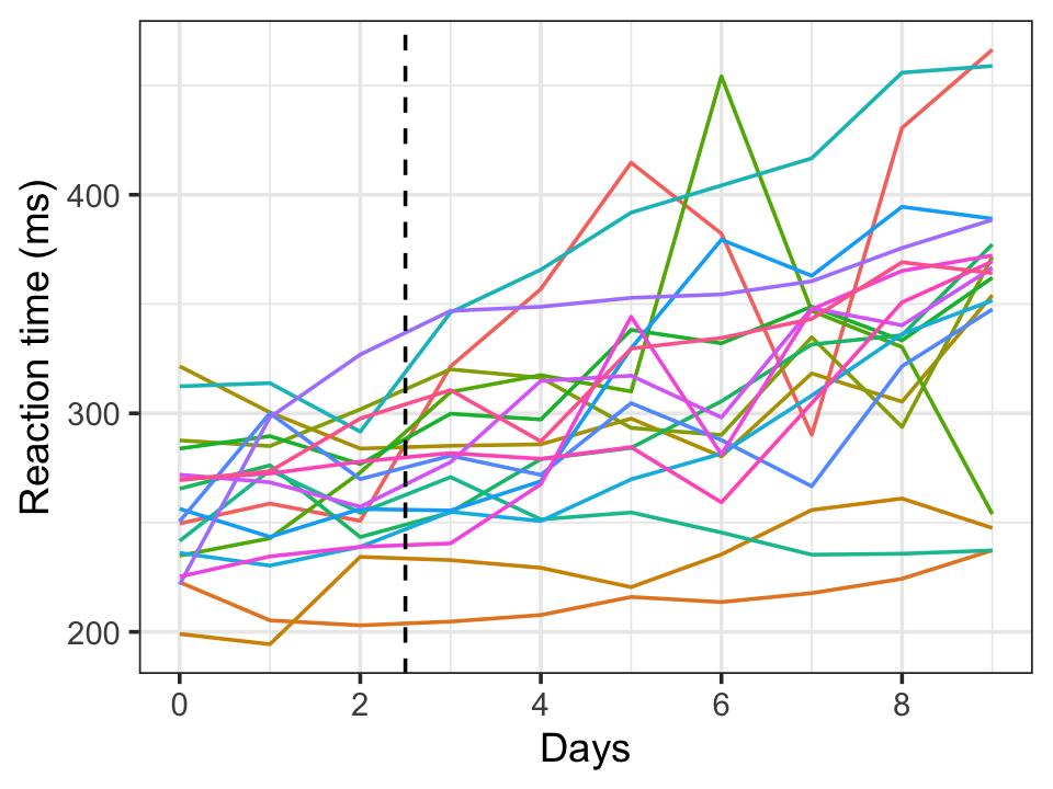
Example 21.11 (Random intercepts and slopes) The data from the sleep deprivation study of Example 21.2 is provided in the lme4 package as sleepstudy. The data is plotted in Figure 21.2, which shows there is a great deal of variation from subject to subject both in baseline reaction time (days 0-2) and in reaction time during sleep deprivation (day 3 onward). Thus it is reasonable to assume each subject has a different intercept and also a different slope (a different reaction to sleep deprivation).

Figure 21.2: Average reaction time in the sleep study. The vertical line indicates the start of sleep deprivation (after day 2). Each line is one experimental subject.

We can do this by including a (Days | Subject) term in the model formula, which tells lmer() to include a random intercept and slope for Days:

sleep_fit <- lmer(Reaction ~ Days + (Days | Subject),
                  data = sleepstudy)
summary(sleep_fit)

Linear mixed model fit by REML ['lmerMod']
Formula: Reaction ~ Days + (Days | Subject)
   Data: sleepstudy

REML criterion at convergence: 1743.6

Scaled residuals: 
    Min      1Q  Median      3Q     Max 
-3.9536 -0.4634  0.0231  0.4634  5.1793 

Random effects:
 Groups   Name        Variance Std.Dev. Corr
 Subject  (Intercept) 612.10   24.741       
          Days         35.07    5.922   0.07
 Residual             654.94   25.592       
Number of obs: 180, groups:  Subject, 18

Fixed effects:
            Estimate Std. Error t value
(Intercept)  251.405      6.825  36.838
Days          10.467      1.546   6.771

Correlation of Fixed Effects:
     (Intr)
Days -0.138

To read the model summary:

The Fixed effects table shows the average intercept and slope. The average subject has a reaction time of about 250 ms on day 0, and their reaction time increases by about 10 ms per day.
The Correlation of Fixed Effects table shows the off-diagonal entries of $\widehat{\var}(\hat \beta)$, i.e., the correlation between $\hat \beta_0$ and $\hat \beta_1$.
The Random effects table shows the variation in intercept between subjects; it has a standard deviation of about 25 ms. It also shows the variation in slope between subjects, which is about 6 ms/day. These estimates have a nonzero correlation with each other.

ranef(sleep_fit)

$Subject
    (Intercept)        Days
308   2.2585510   9.1989758
309 -40.3987381  -8.6196806
310 -38.9604090  -5.4488565
330  23.6906196  -4.8143503
331  22.2603126  -3.0699116
332   9.0395679  -0.2721770
333  16.8405086  -0.2236361
334  -7.2326151   1.0745816
335  -0.3336684 -10.7521652
337  34.8904868   8.6282652
349 -25.2102286   1.1734322
350 -13.0700342   6.6142178
351   4.5778642  -3.0152621
352  20.8636782   3.5360011
369   3.2754656   0.8722149
370 -25.6129993   4.8224850
371   0.8070461  -0.9881562
372  12.3145921   1.2840221

with conditional variances for "Subject"

Example 21.12 (European protected ham) TODO https://cmustatistics.github.io/data-repository/money/european-ham.html

21.6 Random effects as shrinkage

Mixed effects models can also be seen as applying a kind of data-dependent penalization, comparable to the penalization of Chapter 19—but instead of shrinking coefficients towards zero, random effects are shrunk toward their mean. The amount of shrinkage depends on the random effect variance, which is estimated during model-fitting, making this an apparently more principled, data-dependent shrinkage than, say, ordinary ridge regression.

The penalization arises from the assumption that random effects come from a normal distribution with mean zero. This is easiest to see algebraically in a simple intercepts-only model.

Example 21.13 (Shrinkage of random intercepts) Consider the model $\Y = \gamma\T \Z + e$, where $e \sim \normal(\zerovec, \sigma^2 I)$. If we treat this as an ordinary least squares model, we would estimate \[ \hat \gamma_\mathrm{OLS} = (\Z\T\Z)^{-1} \Z\T \Y, \] following the derivations in Chapter 5. If we use ridge regression, we would estimate \[ \hat \gamma_\mathrm{ridge} = (2n \lambda I + \Z\T\Z)^{-1} \Z\T\Y, \] following Section 19.2. If we instead assume $\gamma \sim \normal(\zerovec, \sigma_\gamma^2 I)$ and use the BLUP of Theorem 21.2, then \[\begin{align*} \hat \gamma_\mathrm{BLUP} &= \hat \Sigma \Z\T \widehat{\var}(\Y)^{-1} \Y\\ &= (\hat \sigma_\gamma^2 I) \Z\T \left(\hat \sigma^2 I + \hat \sigma_\gamma^2 \Z\Z\T\right)^{-1} \Y\\ &= \Z\T \left( \frac{\hat \sigma^2}{\hat \sigma_\gamma^2} I + \Z\Z\T\right)^{-1} \Y\\ &= \left(\frac{\hat \sigma^2}{\hat \sigma_\gamma^2} I + \Z\T\Z\right)^{-1} \Z\T \Y, \end{align*}\] using the cyclic permutation property of transposes and the symmetry of the inverse. This looks like the ridge regression estimator!

Just as ridge shrinks the coefficients toward zero, the BLUP estimates shrink toward zero, with the amount of shrinkage determined by the estimates of the variance components ($\hat \sigma^2$ and $\hat \sigma_\gamma^2$), which play a role similar to $\lambda$ in the ridge regression estimator. When $\hat \sigma_\gamma^2 \gg \hat \sigma^2$, the variance due to the random effects dominates and the estimate is close to the OLS estimate; when $\hat \sigma_\gamma^2 \ll \hat \sigma^2$, the variance is mainly due to noise ($e$), and the estimates are heavily penalized.

While the parallel with ridge regression is illuminating, the situation gets far more complicated when we have fixed effects and random effects for both slopes and intercepts. There is no longer an easy formula for the shrinkage, but the shrinkage effect still exists. We can see this graphically by considering a more complicated random effects model.

Example 21.14 (Simulated shrinkage) Suppose observations come from $K$ groups, and each group has its own slope and intercept, so that \[ Y_i = \beta_{0, \text{group}[i]} + \beta_{1, \text{group}[i]} X_i + e_i, \] where $\text{group}[i]$ is the group index of observation $i$. We can fit this data in two different ways. First, we could allow fixed effects per group and an interaction between group and $X$. This model would have $2K$ parameters, a slope and intercept per group, plus the residual variance parameter $\sigma^2$. Alternately, we could allow for random intercepts and slopes per group, as well as a fixed intercept and slope. This model would have $2 + 2 = 4$ parameters (slope, intercept, and variance for each random effect), plus the residual variance parameter $\sigma^2$.

In lmer() formula notation, the two models are:

y ~ x * group
y ~ x + (x | group)

In this simulation, we have $K = 26$ groups labeled A-Z. Each group has a random slope and intercept, drawn from normal distributions. There is an overall average intercept of 4 and slope of 7. We draw $n = 500$ observations and fit both fixed and random effects models:

groups <- LETTERS

group_means <- rnorm(26, sd = 0.5)
names(group_means) <- groups

group_slopes <- rnorm(26, sd = 0.5)
names(group_slopes) <- groups

shrink_pop <- population(
  group = predictor(rfactor, levels = groups),
  x = predictor(rnorm),
  y = response(
    4 + by_level(group, group_means) +
      x * (7 + by_level(group, group_slopes)),
    error_scale = 1
  )
)

shrinks <- shrink_pop |>
  sample_x(n = 500) |>
  sample_y()

shrink_fit <- lm(y ~ group * x, data = shrinks)
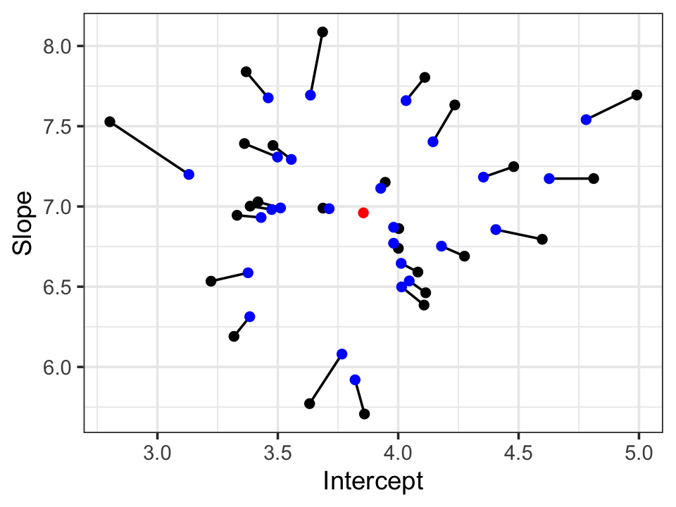
shrink_lmer <- lmer(y ~ x + (x | group), data = shrinks)

From these models, we can extract the slope and intercept per group. These are plotted in Figure 21.3. We can see that the random effects estimates are shrunk toward the overall mean. The amount of shrinkage is proportional to the distance from the mean, so groups already close to the mean receive less shrinkage than the outlying groups.

Figure 21.3: Shrinkage of slopes and intercepts in random effects models (blue) compared to fixed effects (black). Each point is the slope and intercept for one group in the model. In the random effects version, the slopes and intercepts shrink toward the mean slope and intercept (in red).

21.7 Diagnostics

In a linear mixed model, we make many of the same assumptions as in an ordinary linear model, and many of the same diagnostic tools from Chapter 9 are available. We also have additional assumptions, such as the assumed distribution of the random effects, and the complicated estimation of mixed models means there are more details to consider.

21.7.1 Residuals

There are several kinds of residuals we can use in linear mixed models, because a mixed model’s sources of variation can be broken into multiple pieces (Hilden-Minton 1995, sec. 4.1):

The conditional error $e$
The random effects $\gamma\T \Z$
The marginal error, $\xi = \gamma\T\Z + e$, which combines the conditional error and random effects

We can define residuals to let us examine each of these sources of variation.

Definition 21.3 (Linear mixed model residuals) In linear mixed model defined as in Definition 21.1, we can define the following residuals:

Conditional residuals: $\hat e = \Y - \hat \beta\T \X - \hat \gamma\T \Z$, where $\hat \gamma$ is estimated with the BLUP (Theorem 21.2), estimating the error term $e$. Also known as case-unique or level-1 residuals
Random effects residuals: $\hat d = \hat \gamma\T Z$, the differences between the population mean for each observation and the prediction conditional on the random effects. Also known as level-2 residuals
Marginal residuals: $\hat \xi = \Y - \hat \beta\T \X$, where the random effects are marginalized out. Also known as composite residuals or the empirical BLUP (EBLUP)

Depending on if we want to check the structure of the mean function, of $e$, or of $\gamma$, different residuals will be useful for each job. Intuitively, the conditional residuals would be used to check that $e$ is normal, mean zero, and has constant variance, as well as identifying outliers; the marginal residuals would be used to check the linearity of the relationship between $\X$ and $\Y$; and the random effects residuals would be used to check the normality of $\gamma$ and to identify outlier random effects.

However, how we do this is more specific than in ordinary linear models, because different kinds of model misspecification are confounded with each other.

Theorem 21.3 (Properties of linear mixed model residuals) A residual is called pure for an error term if its form depends only on that error. A residual is confounded for an error term if it also depends on other error terms. For example,

The conditional residuals are confounded for the conditional error $e$
The random effects residuals are confounded for the random effects $\gamma\T\Z$
The marginal residuals $\hat \xi$ are pure for the marginal error $\xi$

Proof. For details, see Hilden-Minton (1995), section 4.1. For intuition,

The conditional residuals are \[\begin{align*} \hat e &= \Y - \hat \beta\T \X - \hat \gamma\T \Z \\ &= \beta\T \X + \gamma\T \Z + e - \hat \beta\T \X - \hat \gamma\T \Z, \end{align*}\] and the BLUP $\hat \gamma$ is defined in terms of $\Y - \X \hat \beta$, which depends on the true $\gamma$. Thus the conditional residuals depend on both $\gamma$ and $e$.
The random effects residuals are \[\begin{align*} \hat d &= \hat \gamma\T \Z \\ &= \left(\hat \Sigma \Z\T \widehat{\var}(\Y)^{-1} (\Y - \X \hat \beta)\right)\T \Z, \end{align*}\] which, again, depends on both $e$ and $\gamma$.
The marginal residuals are \[\begin{align*} \hat \xi &= \Y - \hat \beta\T \X \\ &= \beta\T \X + \gamma\T \Z + e - \hat \beta\T \X, \end{align*}\] which depends on $\gamma\T \Z + e = \xi$, the marginal error. As $\X$ is fixed, the marginal residuals have no other source of error.

Residual confounding makes it difficult to uniquely attribute a problem to a single source. For example, if the conditional residuals are non-normal, it is not obvious if that is because the errors $e$ are non-normal or because the random effects $\gamma$ have an unusual distribution. The residuals will have to be considered collectively to narrow down the problem.

To compute the residuals, we will use the HLMdiag package (Loy and Hofmann 2014), which produces residual diagnostics in tidy format for a variety of mixed-effect model types. Its hlm_resid() function augments the model data frame with additional columns for residuals and fitted values, making it easy to construct residual diagnostic plots.

21.7.2 Mean function misspecification

As in ordinary linear regression, it is important to check if the relationship between $X$ and $Y$ is linear. Marginally, our model assumes that $\E[Y \mid X = x] = \beta\T x$, even in a mixed model, so we must check this assumption. All of the same considerations from ordinary linear models (discussed in Section 9.2) apply to mixed models as well. As we are interested in the marginal relationship between $X$ and $Y$, it makes sense to use the marginal residuals.

Example 21.15 (Marginal residuals in the sleep study) In the sleep study of Example 21.11, we can use hlm_resid() to obtain a data frame whose .mar.resid column contains the marginal residuals:

library(HLMdiag)

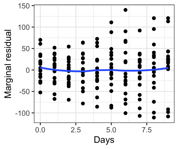
sleep_mar_resids <- hlm_resid(sleep_fit)

The fixed effect is Days, so plotting these against Days will reveal any misspecification. As with other residual plots, including a smoothing line is often helpful. Figure 21.4 shows the result, which does not indicate any problems with the mean function. The error variances do appear to increase with Days, but these residuals are not standardized and also depend on the random effects, so this is not a definitive sign of heteroskedasticity in $e$. We will consider error variance checks in Section 21.7.3.

Figure 21.4: Marginal residuals vs. days in the sleep study.

21.7.3 Error misspecification

To check that the errors $e$ have constant variance and are normally distributed, it makes sense to use the conditional residuals $\hat e$, even though they are confounded. These can be standardized by their estimated variance, permitting us to visually diagnose heteroskedasticity and non-normality. We can also identify potential outliers needing investigation.

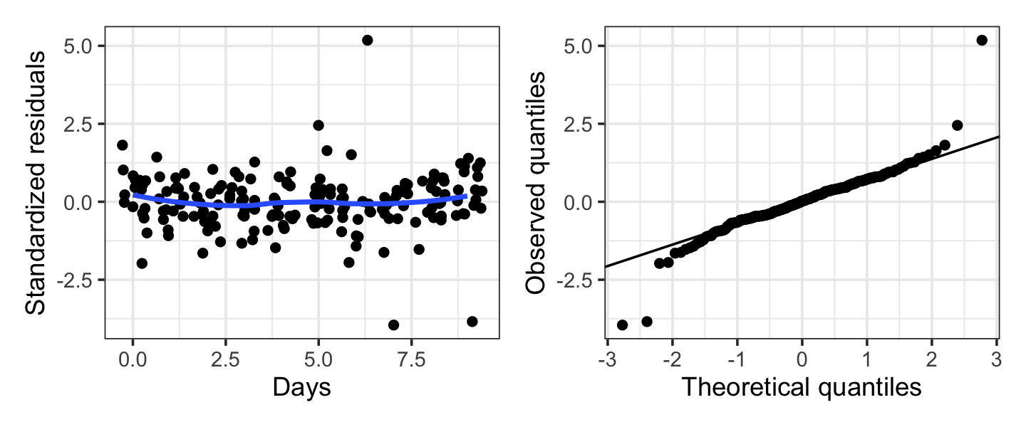
Example 21.16 (Error diagnostics in the sleep study) In the sleep study of Example 21.11, we can use hlm_resid() with standardize = TRUE to obtain the standardized conditional residuals in the .std.resid column:

sleep_cond_resids <- hlm_resid(sleep_fit, standardize = TRUE)

The resulting diagnostic plots are shown in Figure 21.5. The errors appear slightly heavy-tailed, but only about a half-dozen observations are involved, so this is not terribly concerning. The variance appears reasonably constant, apart from the few outlying residuals. By identifying the observations with these outlying residual values, we can investigate the outliers and determine if they are problems.

Figure 21.5: *Left*: Standardized conditional residuals, jittered so the variance is easier to see. *Right:* Q-Q plot of standardized conditional residuals, showing slightly heavy tails.

21.7.4 Random effect misspecification

TODO

21.7.5 Outliers and influential observations

TODO

21.8 Bayesian hierarchical models

TODO

Exercises

Exercise 21.1 (Choose a suitable mixed model) For each of the following situations, choose a suitable mixed model to use and specify it in lme4’s formula syntax. For each random effect, state why you modeled it as random. You do not need to use every variable provided. Assume every relationship is linear.

In an educational study, we enroll third-grade students in Burpleson Elementary School in a study of the effect of laptops on student learning. Half of students are provided a laptop with electronic textbooks, the other half are provided physical textbooks. At the end of the school year, all students take the state standardized Evaluation of Vocational and Informational Literacy test, which measures their reading ability. Each row of data is a student, with the following variables:
- id: Student ID number
- treatment: Factor indicating whether they received a laptop or textbooks
- teacher: Factor indicating their reading teacher’s name
- evil: EVIL score at the end of the year
Select a model to estimate the effect of laptop or textbook use on reading ability.
In a sports study, we track the performance of runners at marathons across the United States. We’re interested in whether the outside air temperature affects the average completion time of runners (perhaps runners can’t sustain high speeds on hotter days). For each marathon, we have data on all runners, as well as the outside air temperature. Many runners participated in multiple marathons, so we have data for them at multiple temperatures. Each row is one runner in one marathon, with the following variables:
- runner: The runner ID
- location: A factor indicating where this marathon is held
- time: The runner’s completion time (seconds)
- temp: The outside air temperature on race day
In a medical study, we enroll patients with high blood pressure. Each patient is assigned a dosage of our experimental blood pressure medication. A week after receiving it, we measure their blood pressure five times (because blood pressure measurements tend to be quite variable). We want to measure the effect of the treatment on blood pressure. Each row of data is a single blood pressure measurement, with the following variables:
- bp: The blood pressure
- patient: A unique patient ID number
- dosage: The amount of medication they received (a factor with four levels)
- measurement_no: Which blood pressure measurement it is, from 1 to 5
- age: Patient age (years), which is thought to be related to blood pressure
Select a model to estimate the effect of dosage on blood pressure.

Exercise 21.2 (Marginal distribution of the mixed model) Using the laws of total expectation and variance, prove Theorem 21.1 by showing that the mixed model \[\begin{align*} \Y \mid \gamma &\sim \normal(\beta\T \X + \gamma\T \Z, \sigma^2 I)\\ \gamma &\sim \normal(\zerovec, \Sigma) \end{align*}\] can be written marginally as \[ \Y \sim \normal(\beta\T \X, \sigma^2 I + \Z \Sigma \Z\T). \] You may assume without proof that if a distribution is conditionally normal, and its mean is marginally normal, the marginal distribution is also normal.

Exercise 21.3 (Marginal likelihood in the random intercepts model) Consider the marginal model in Theorem 21.1 applied to the random intercepts model of Example 21.3. Based on the structure of $\Z$ and the variance in Example 21.5, describe the structure of the marginal variance matrix $\var(\Y)$. Show it matches the variance described in Example 21.7.

Exercise 21.4 (Mixed model diagnostics) The following regressinator population has observations in groups A through Z, but several mixed-effects model assumptions are violated:

groups <- LETTERS

group_means <- rnorm(26, sd = 0.5)
names(group_means) <- groups

group_slopes <- rt(26, df = 3) * 0.5
names(group_slopes) <- groups

misspec_pop <- population(
  group = predictor(rfactor, levels = groups),
  x = predictor(rnorm),
  y = response(
    4 + by_level(group, group_means) +
      x * (7 + by_level(group, group_slopes)) + 0.3 * x^2,
    family = ols_with_error(rt, df = 3),
    error_scale = 1
  )
)

Consider fitting a linear mixed-effects model to this data where we assume $X$ is linearly related to $Y$.

Give the model formula for a model that would, if the assumptions were met, be appropriate for this data.
List the mixed-effects model assumptions that are violated in this dataset.
Draw a sample of $n = 500$ observations and fit the mixed-effects model. Plot the marginal, conditional, and random effects residuals following the procedures shown in Section 21.7. For each plot, comment on what it shows, and which, if any, assumption violations are visible in it.

Exercise 21.5 (Cupping marks) TODO replicate analysis in https://stat.columbia.edu/~gelman/research/unpublished/healing.pdf

Exercise 21.6 (Stress and cognitive effort) TODO https://cmustatistics.github.io/data-repository/psychology/stress-effort.html

Exercise 21.7 (Productivity gains from using AI) As generative AI tools became popular, many software companies argued that software developers can be more productive when they use AI tools to help them write code. Claims about productivity are always hard to verify. The CMU S&DS Data Repository contains a dataset from an experiment by METR, an independent AI research group, that randomly assigned developers to either use AI or not use AI to complete tasks, then assessed the time taken to complete each task. Each developer completed multiple tasks, some with AI and some without.

Review the data description. Then:

Conduct an exploratory data analysis to see how much variation there is between developers and how much a difference in implementation time there is between AI and no-AI conditions.
Select an appropriate model to estimate the effect of AI use on the initial implementation time for each task. Explain and justify your choices.
Fit your chosen model. Conduct a residual analysis and comment on the model assumptions. Are there any signs of misspecification? If so, propose a revised model.
Using your final model, interpret the result: does AI reduce the time developers take to complete tasks?