18  Estimating Error

\[ \DeclareMathOperator{\E}{\mathbb{E}} \DeclareMathOperator{\R}{\mathbb{R}} \DeclareMathOperator{\RSS}{RSS} \newcommand{\X}{\mathbf{X}} \newcommand{\Y}{\mathbf{Y}} \newcommand{\T}{^\mathsf{T}} \DeclareMathOperator{\var}{Var} \DeclareMathOperator{\cov}{Cov} \DeclareMathOperator{\edf}{edf} \DeclareMathOperator{\AIC}{AIC} \DeclareMathOperator{\se}{se} \newcommand{\trainset}{\mathcal{T}} \DeclareMathOperator{\normal}{Normal} \DeclareMathOperator*{\argmax}{arg\,max} \]

If we cannot use the training error to identify the model with the best generalization error, and hence the best prediction performance, how should we select models? Evidently we need estimators for the generalization error. There are many options, starting with simple formulas and advancing to computationally intensive procedures that can be adapted to almost any setting. But the estimators aren’t enough: we’ll also need a coherent strategy for selecting models.

18.1 Shortcut estimators

The simplest approach for estimating generalization error draws directly from Theorem 17.3. If the training error is, on average, too small by an amount we can estimate, we could “de-bias” it by adding that back to the training error. This estimates the in-sample prediction error (Definition 17.6).

For example, in Example 14.3, we showed that the effective degrees of freedom for a linear regression model with \(p\) regressors is simply \(\edf(\hat f) = p\). Rearranging the optimism formula, we obtain \[ \E[R_\text{in}] = \E[R_\text{train}] + \frac{2 \sigma^2}{n} p. \] We can estimate \(\sigma^2\) with \(S^2\) (Theorem 5.2) and estimate \(\E[R_\text{train}]\) with the observed \(R_\text{train}\). This leads to Mallows’s \(C_p\) statistic (Gorman and Toman 1966).

Definition 18.1 (Mallows’s \(C_p\)) The Mallows’s \(C_p\) statistic for a linear regression model with \(p\) predictors is \[ C_p = \frac{\RSS}{n} + \frac{2 p S^2}{n}. \] When comparing multiple linear models of different sizes, it is common to use the largest model to estimate \(S^2\) and use that value to calculate \(C_p\) for the other models.

This definition only applies to linear models, not generalized linear models, due to its dependence on \(S^2\). But by the same argument, we can construct an estimator of the test log-likelihood for any log-likelihood-based model (Theorem 17.4).

Definition 18.2 (Akaike Information Criterion) The Akaike Information Criterion (AIC) for a model with log-likelihood \(\ell(\hat \beta)\) and \(p\) parameters is \[ \AIC = - \frac{2}{n} \ell(\hat \beta) + 2 \frac{p}{n}. \]

In linear models with normally distributed errors, this is equivalent to Mallows’s \(C_p\) (Exercise 18.1). Either criterion can be used to select from a set of models fit to the same training data: calculate \(C_p\) or AIC for all of the models and select the model with the smallest value of \(C_p\) or AIC. (Note that some books or programs define \(C_p\) and AIC with different signs, so you may want the largest value—check the definition before you confuse yourself.)

As the AIC can be used for any model with a log-likelihood, you will see it used in many different contexts, particularly when cross-validation would be inconvenient because the model is slow to fit.

18.2 Sample splitting

The next option is to divide our data into several pieces. For instance, we might split into two sets: the training set and the test set. We use the training set to estimate the model parameters, then evaluate the loss on the test set. In the notation of Chapter 17, divide the dataset \(\trainset\) into two sets \(\trainset_\text{train}\) and \(\trainset_\text{test}\), then evaluate: \[\begin{align*} \hat \beta &= \argmax_\beta \ell(\beta, \trainset_\text{train}) \\ \hat R &= \frac{1}{n_\text{test}} \sum_{i \in \trainset_\text{test}} L(y_i, \hat f(x_i)). \end{align*}\]

Typically the split is done randomly. The proportion to place in each set is a matter of taste: you will often see 50/50 train/test splits, but also 75/25, 60/40, and various other proportions.

This approach is simple and easy to implement for various loss functions \(L\). If we are considering several models, we can choose the model whose estimated generalization error \(\hat R\) is the smallest.

However, there are several complications:

1. Because we are fitting \(\hat \beta\) to \(\trainset_\text{train}\), which is smaller than \(\trainset\), our model will have higher variance than it would on the entire dataset. Our estimate \(\hat R\) will hence likely overestimate the prediction error.
2. Because the estimate \(\hat R\) is based on a random split, it has its own variance: repeat the procedure with the same model on the same data \(\trainset\), but with different train/test splits, and you will obtain different results. If you are ranking several models using \(\hat R\), you may obtain different rankings each time.
3. It’s not entirely obvious which error from Chapter 17 we’re estimating: we’re not estimating the generalization error \(R_{\trainset}\) (Definition 17.2) because we’re fitting only on \(\trainset_\text{train}\), not \(\trainset\); we’re not estimating the in-sample prediction error \(R_\text{in}\) (Definition 17.6) because we’re not testing at identical \(X\) values; are we estimating the expected generalization error \(R\) (Definition 17.3)?

Before we resolve these questions, we can consider a straightforward improvement of sample splitting: cross-validation.

18.3 Cross-validation

Cross-validation extends the idea of sample splitting. If we split the dataset into pieces, training on one and testing on another, can we then swap their roles and evaluate the model again? That would allow us to average the estimates, perhaps reducing the variance and producing a better estimate.

18.3.1 K-fold cross-validation

The K-fold cross-validation procedure implements this basic sample splitting idea.

Definition 18.3 (K-fold cross-validation) To estimate the prediction error of a model \(\hat f(x)\), randomly split the available dataset \(\trainset\) into \(K\) folds \(\trainset_1, \trainset_2, \dots, \trainset_K\). (If the dataset is not evenly divisible by \(K\), these may not be exactly the same size.) Then:

1. Fit \(\hat f(x)\) using \(\trainset_2, \trainset_3, \dots, \trainset_K\) as the training data.
2. Evaluate the average loss \(L\) on \(\trainset_1\) to obtain \(\hat R_1\).
3. Repeat steps 1 and 2 a total of \(K\) times, each time fitting \(\hat f(x)\) to \(K - 1\) of the folds and evaluating the loss on the remaining fold, to obtain \(\hat R_1, \dots, \hat R_K\).
4. Report the average of \(\hat R_1, \dots, \hat R_K\) as the estimated prediction error.

While this procedure requires us to fit the model \(K\) times, which may be inconvenient when the model is slow to fit, it has several advantages over basic sample splitting:

1. Each model \(\hat f(x)\) is fit to \(n (K - 1) / K\) observations, which is often more than the equivalent model in sample splitting. For instance, in 10-fold cross-validation, each model is fit using 90% of the data, while in a 60/40 train/test split the model would only use 60% of the data. Hence the prediction variance will be less of an overestimate.
2. Because the estimate is repeated \(K\) times and averaged, it should have lower variance than a single error estimate, and will have better accuracy (Blum, Kalai, and Langford 1999).

Typically, \(K\) is 5, 10, or 20. There’s no reason to mess around trying different values. Just pick, say, \(K = 10\) and stick with it.

Example 18.1 (Cross-validation in R) For easy cross-validation in R, we can use the rsample package again, as we did with bootstrapping. rsample calls K-fold CV “V-fold cross-validation”, but it’s the same thing.

As in Exercise 17.1, let’s imagine fitting a smoothing spline to the Doppler function and estimating it’s error. We have one sample from the population, doppler_samp, and we want to fit a spline with 7 degrees of freedom:

fit <- smooth.spline(doppler_samp$x, doppler_samp$y, df = 7)

How can we estimate the error? Let’s use vfold_cv() from rsample to get 10 folds:

library(rsample)

folds <- vfold_cv(doppler_samp, v = 10)
folds

#  10-fold cross-validation 
# A tibble: 10 × 2
   splits          id    
   <list>          <chr> 
 1 <split [90/10]> Fold01
 2 <split [90/10]> Fold02
 3 <split [90/10]> Fold03
 4 <split [90/10]> Fold04
 5 <split [90/10]> Fold05
 6 <split [90/10]> Fold06
 7 <split [90/10]> Fold07
 8 <split [90/10]> Fold08
 9 <split [90/10]> Fold09
10 <split [90/10]> Fold10

Each row of folds is one train/test split. The splits column contains the splits. For each split, we can fit our model on the training (“analysis”) data and test it on the test (“assessment”) data:

errors <- sapply(folds$splits, function(split) {
  train <- analysis(split)
  test <- assessment(split)

  fit <- smooth.spline(train$x, train$y, df = 7)

  test_predictions <- predict(fit, test$x)$y

  mean((test_predictions - test$y)^2)
})

mean(errors)

[1] 0.07954361

This estimate is random: the 10 folds are selected by randomly splitting the data, and if we repeated the process, we’d get 10 different folds and 10 different error estimates. We can estimate the variability of the process by noting the variability in the 10 error estimates we obtained:

errors

 [1] 0.01032977 0.12492713 0.06763923 0.09050913 0.10876057 0.07635989
 [7] 0.06397506 0.07743478 0.10356831 0.07193221

The largest and smallest errors differ by a factor of 12. (This is partly because our sample has size \(n = 100\), and so in 10-fold cross-validation, each test set is of size 10; if the data were larger, or we used fewer folds, each error estimate would be the average error on a larger test set.)

18.3.2 Leave-one-out cross-validation

If K-fold cross-validation fits the model on all but \(1/K\)th of the data, using the left-out piece to evaluate it, we might ask: can we fit on all but one observation?

Definition 18.4 (Leave-one-out cross-validation) To estimate the prediction error of a model \(\hat f(x)\) using \(n\) observations,

1. Fit \(\hat f(x)\) using \(\{(x_1, y_1), (x_2, y_2), \dots, (x_{n - 1}, y_{n - 1})\).
2. Evaluate the loss \(L(y_n, \hat f(x_n))\).
3. Repeat steps 1 and 2 a total of \(n\) times, each time fitting \(\hat f(x)\) to all but one observation and evaluating the loss on the remaining observation.
4. Report the average loss on all \(n\) held-out observations as the estimated prediction error.

This procedure—often called LOO or LOOCV—has several advantages over K-fold cross-validation:

1. Each model \(\hat f(x)\) is fit to \(n - 1\) observations. When \(n\) is large, this is a negligible difference in sample size, so each model has about the same variance as a model fit to the full data.
2. There is no random splitting: given the same training data, LOOCV will obtain the same error estimate every time.

Perhaps most importantly, there are special cases when LOOCV does not require actually refitting the model \(n\) times—the error can be estimated in closed form from the fitted model.

Example 18.2 (LOOCV in linear models) Consider a linear model fit to \(n\) observations using the squared-error loss. The LOOCV estimate of prediction error is equal to \[ \hat R_\text{loocv} = \frac{1}{n} \sum_{i=1}^n \frac{\hat e_i^2}{(1 - H_{ii})^2}, \] where \(H_{ii}\) is the leverage of observation \(i\) and \(\hat e_i\) is the residual. Fitting the model \(n\) times is not necessary; only the residuals and leverages from the model fit to the entire dataset is needed.

The argument is the same as for the formula for Cook’s distance (Theorem 9.1): we can use the leverage to obtain \(\hat \beta^{(i)}\), the fit when observation \(i\) is omitted, so we can use it to obtain the error in predicting observation \(i\) when it is not used to fit the model. (For details, see Seber and Lee (2003), pages 403–404.)

In other models, there may be approximate formulas for LOOCV error with specific loss functions. These formulas were valuable in the early days of statistical computing, when re-fitting models could be very slow, and are still useful when fitting models on enormous datasets.

On the other hand, LOOCV has a drawback: while it does average together \(n\) error estimates, those estimates are highly correlated with each other, and so the resulting prediction error estimate has high variance. The high correlation is because each \(\hat f(x)\) shares nearly all of its training observations with every other \(\hat f(x)\) fit during the procedure. As a result, Hastie, Tibshirani, and Friedman (2009) (section 7.10) recommend 5- or 10-fold cross-validation as reasonable defaults.

18.3.3 What error does cross-validation estimate?

By this point, the astute reader may have noticed I have not answered Chekhov’s statistical question in Section 18.2: Which type of error does cross-validation estimate? Does it estimate the generalization error \(R_{\trainset}\), the in-sample prediction error \(R_\text{in}\), or the expected generalization error \(R\)?

This question is surprisingly difficult to answer. Ideally, we could estimate \(R_{\trainset}\): the prediction error of our model fit to this specific training set \(\trainset\). As every cross-validation estimator uses \(\trainset\) to obtain its estimate, it seems like cross-validation should estimate \(R_{\trainset}\)—but it does not. Indeed, the correlation between the cross-validation error and \(R_{\trainset}\) (across different samples \(\trainset\) from the population) is roughly zero.

Bates, Hastie, and Tibshirani (2024) show that in linear models, cross-validation is a better estimate of the expected generalization error \(R\) than it is of \(R_{\trainset}\). Recall that \(R = \E[R_{\trainset}]\), so cross-validation is a better estimate of how this model will behave on average, given any sample from the population, than it is of how well this model performs when fit on our specific \(\trainset\). It is a biased estimate because the models in cross-validation are fit to \(n(K - 1) / K\) observations instead of \(n\), and hence have higher variance than a model fit to the full data, but we will see that the bias is less important when we are using cross-validation to select models.

18.3.4 Uncertainty in cross-validation errors

Since cross-validation is an estimator (of something), it is reasonable to ask for its uncertainty. We could use this when comparing several models to find the one with the best prediction performance: if the uncertainty is high, we may be less confident in our selection than if the uncertainty is small.

\(K\)-fold cross-validation produces \(K\) individual error estimates that are averaged; LOOCV produces \(n\) individual estimates. We could use their variability to estimate the uncertainty. In intro stats, if we have \(K\) samples from some population and use their sample mean to estimate the population mean, the standard error of the mean is the standard deviation (of the \(K\) samples) divided by the square root of the sample size (\(K\)).

It stands to reason, then, that if we have \(K\) estimates \(\hat R_1, \hat R_2, \dots, \hat R_K\), we could obtain the standard error \[ \se(\hat R) = \frac{1}{K} \sqrt{\widehat{\var}(\hat R_1, \dots, \hat R_K)}, \] where \(\widehat{\var}\) is the sample variance function.

However, in intro stats, our \(K\) samples are independent samples from the population. Here, the cross-validation error estimates are not independent, as they are based on fits to overlapping samples. This standard error is hence generally an underestimate; you can’t use it to, say, construct a valid 95% confidence interval for the expected prediction error \(R\). Unfortunately, there is no unbiased estimator of the variance of \(\hat R\) using only \(\hat R_1, \dots, \hat R_K\) (Bengio and Grandvalet 2004); the only unbiased estimates involve repeating cross-validation several times, such as the nested procedure suggested by Bates, Hastie, and Tibshirani (2024).

Nevertheless, the simple cross-validation standard errors are widely used. They at least provide a simple way to guesstimate whether an observed difference between two models is large or close to the noise, even if they cannot provide a formal inference procedure.

18.3.5 Order of operations in cross-validation

If cross-validation is thought of as estimating the model’s performance given any sample from the population, we must consider the model fitting procedure as a whole. For example, suppose we fit a model that depends on some kind of tuning parameter, like the smoothness parameter in additive models (Chapter 14) or the penalty parameter in penalized models (to be introduced in Chapter 19). We might fit the model using the following procedure:

1. Use the data in some kind of procedure to choose the “best” tuning parameter. (Often this procedure involves using cross-validation to try different values.
2. Fit the model using the selected tuning parameter values.
3. Use cross-validation on the final model to estimate its prediction error.

Or suppose we want to use some kind of model-selection procedure to reduce the number of variables in the model, using the following procedure:

1. Use stepwise selection, \(F\) tests, or some other model selection procedure on the full dataset to pick out the “best” variables.
2. Fit the model using the selected variables.
3. Use cross-validation on the final model to estimate its prediction error.

Unfortunately, these procedures will always give us the wrong answer, as we can see in a trivial example.

Example 18.3 (Order of operations in cross-validation) Let’s consider a population where the true values of \(R\), \(R_{\trainset}\), and \(R_\text{in}\) are trivial: one where \(Y \sim \normal(0, 1)\), independent of \(X\). There are \(p = 500\) predictors that are all standard normal, and they are all equally useless.

library(regressinator)
library(mvtnorm)

cv_pop <- population(
  x = predictor(rmvnorm, mean = rep(0, 500)),
  y = response(0, error_scale = 1)
)

cv_samp <- cv_pop |>
  sample_x(n = 100) |>
  sample_y()

We have \(n = 100\) observations but \(p = 500\) predictors, so let’s imagine we’re using forward stepwise selection to select fewer than 100 predictors. We’ll discuss forward stepwise in more detail in Definition 19.1, but it’s sufficient for now to say that we add variables one at a time based on those that improve the model’s AIC the most:

# start with only an intercept
initial_fit <- lm(y ~ 1, data = cv_samp)

# add predictors one at a time based on AIC
selected_fit <- step(initial_fit,
                     scope = formula(lm(y ~ ., data = cv_samp)),
                     direction = "forward", trace = 0,
                     steps = 25)

Here I’ve limited the procedure to add only 25 predictors at most. Despite all the predictors being useless, it has selected 25 that “improved” the model’s AIC when they were added.

Because this is a linear model, we can calculate the LOOCV error exactly using Example 18.2:

sum(residuals(selected_fit)^2 /
      (1 - hatvalues(selected_fit))^2) / 100

[1] 0.1800682

But because \(Y \sim \normal(0, 1)\), the best possible prediction error (\(R\), \(R_{\trainset}\), or \(R_\text{in}\)) for any model is 1, for the model that predicts \(\hat Y = 0\). Our model cannot do better than this, so our LOOCV estimate dramatically underestimates the true prediction error.

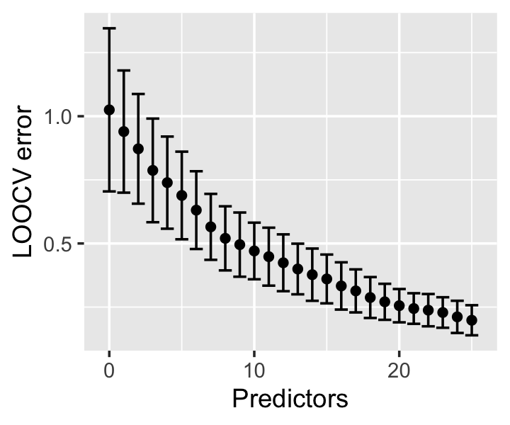
In Figure 18.1 we can see the effect as predictors were added: the initial model, with only an intercept, has a LOOCV error estimate very close to the truth. But as predictors are added based on their predictive performance, we essentially overfit to predictive performance, decreasing the LOOCV error estimate even as the additional predictors add no new predictive ability.

Figure 18.1: LOOCV error estimates as additional (useless) predictors are added. When there are no predictors (only the intercept), the LOOCV estimate is very close to the true irreducible error of 1. Error bars indicate plus or minus two standard errors, as described in Section 18.3.4.

There are two ways to think of the cause of this problem. First, if our initial tuning or model selection uses all the data, we pick a model that works well on all the data—so when part of the data is set aside as a “test” set during the final cross-validation step, it has already been used in training. The held-out test sets haven’t actually been held out, and they no longer represent independent test samples from the population. If we overfit to the full dataset, cross-validation will produce an error estimate reflecting that overfitting.

Alternately, if cross-validation is meant to estimate the expected generalization error \(R\) across training sets, we must cross-validate the whole procedure, including everything that would change if we changed training sets. If a new training set would mean a different selected model or different tuning parameters, that must be part of the cross-validation process. Instead of doing your tuning or selection once, on the entire dataset, you must do it \(K\) times, using only the \(K-1\) folds in each step of your \(K\)-fold cross-validation.

In short: if you build your predictive model using an elaborate procedure of many steps, including various tuning and selection processes, you must cross-validate the entire procedure or your error estimates will likely be far too low. Unfortunately this can be slow if your tuning and selection steps are computationally intensive; and unfortunately, many published papers make this mistake and hence present unreasonably optimistic results.

18.4 The model selection process

As we have seen, cross-validation provides a biased estimate of the expected generalization error. However, the biased estimate can still be useful. Often we are using cross-validation not solely to estimate \(R\) but for model selection: we have several candidate models and would like to select one that is likely to generalize the best to new data. For instance:

1. We’ve fit models with different combinations of predictors
2. We’ve fit simple linear models but also models with interactions, splines, smoothers, etc., and don’t want to overfit
3. We can fit a model with a tuning parameter (e.g. a smoothing spline with its penalty \(\lambda\), Theorem 14.1), and want to pick the best value of the tuning parameter

These scenarios happen all the time, and if our goal is to select the model with the best (expected) generalization error, cross-validation seems plausible. A standard approach is to cross-validate all the candidate models and select the model with the best estimated error.

Here the bias seems less important: each candidate model’s estimate is biased in (roughly) the same way, so comparisons between models should still be reasonable. Cross-validation is hence widely used for model selection, and generally works fairly well to pick a reasonable model, provided the cross-validation has been implemented correctly.¹

18.5 Exercises

Exercise 18.1 (\(C_p\) and AIC) Show that in a normal linear regression model, where \(Y = X\beta + e\) and \(e \sim \normal(0, \sigma^2)\) with \(\sigma^2\) a known constant, the AIC (Definition 18.2) is equal to Mallows’s \(C_p\) (Definition 18.1), up to constants that do not depend on \(X\) or \(Y\).

(When \(\sigma^2\) is a known constant, we can use it in place of \(S^2\) in \(C_p\).)

Exercise 18.2 (College Scorecard) Let’s return to the College Scorecard data from Exercise 11.7. We previously used \(F\) tests to determine if polynomial terms were warranted. But suppose we were instead interested in predicting earnings after graduation, and simply wanted the fit that gave the best predictions.

Use 10-fold cross-validation to estimate the squared-error loss of each of your models from Exercise 11.7. Compare the results to what you got using \(F\) tests. Why could the results differ?

Exercise 18.3 (Abalone weights) Abalone are a type of sea snail often harvested and sold for food. The data file abalonemt.csv (on Canvas) contains nine variables measured on 4173 abalones.

You might want to predict the weight of the edible part of the abalone (Shucked.weight) before shucking it (removing it from its shell), so you can determine how much to charge for the abalone you are selling. You can easily measure the exterior dimensions without shucking it, so you can use the Diameter, Length, and Height predictors.

It might be reasonable to assume the abalone’s weight is proportional to its volume, so that \[ \text{weight} \propto \text{diameter} \times \text{length} \times \text{height}. \] If so, then \[ \log(\text{weight}) \propto \log(\text{diameter}) + \log(\text{length}) + \log(\text{height}). \] Consider several models to predict shucked weight from dimensions:

1. A linear model predicting shucked weight from diameter, length, and height.
2. A linear model predicting \(\log(\text{shucked weight})\) from the log of each dimension.
3. A smoothing spline model (fit with smoothing.spline(), letting it choose the optimal smoothness automatically) predicting shucked weight from the product of diameter, length, and height.

If this model is to be used for pricing, what matters is that it predicts accurately, so customers do not feel ripped off. Use 10-fold cross-validation to estimate the error of each model. Comment on the results. Which model appears best?

When estimating the error of model 2, ensure you measure the squared error for shucked weight, not \(\log(\text{shucked weight})\). You will need to exponentiate its predictions so they are on the same scale as the other models.

Bates, Stephen, Trevor Hastie, and Robert Tibshirani. 2024. “Cross-Validation: What Does It Estimate and How Well Does It Do It?” Journal of the American Statistical Association 119 (546): 1434–45. https://doi.org/10.1080/01621459.2023.2197686.

Bengio, Yoshua, and Yves Grandvalet. 2004. “No Unbiased Estimator of the Variance of K-Fold Cross-Validation.” Journal of Machine Learning Research 5: 1089–1105. https://jmlr.csail.mit.edu/papers/v5/grandvalet04a.html.

Blum, Avrim, Adam Kalai, and John Langford. 1999. “Beating the Hold-Out: Bounds for K-Fold and Progressive Cross-Validation.” In Proceedings of the Twelfth Annual Conference on Computational Learning Theory, 203–8. https://doi.org/10.1145/307400.307439.

Gorman, J. W., and R. J. Toman. 1966. “Selection of Variables for Fitting Equations to Data.” Technometrics 8 (1): 27–51. https://doi.org/10.2307/1266260.

Hastie, Trevor, Robert Tibshirani, and Jerome Friedman. 2009. The Elements of Statistical Learning: Data Mining, Inference, and Prediction. 2nd ed. Springer. https://hastie.su.domains/ElemStatLearn/.

Lei, Jing. 2020. “Cross-Validation with Confidence.” Journal of the American Statistical Association 115 (532): 1978–97. https://doi.org/10.1080/01621459.2019.1672556.

Seber, George A. F., and Alan J. Lee. 2003. Linear Regression Analysis. 2nd ed. Wiley. https://doi.org/10.1002/9780471722199.

---

1. The theoretical development is more complicated: cross-validation is not a consistent model selection procedure, in that it is not guaranteed to select the best model as \(n \to \infty\). There are extensions that are consistent, such as Lei (2020), but they tend to be much more complex. Cross-validation is a good example of a technique that isn’t optimal, but is good enough.