20 Kernel Regression

Hastie, Tibshirani, and Friedman (2009), chapter 6; 402 lec 1 & 7

Penalized regression allows us to adapt our classic linear regression and generalized linear models to higher-dimensional problems, and to trade off bias and variance to improve our prediction performance.

In a pure prediction problem, another approach might be to start out with a more flexible model from the beginning, instead of adapting a linear model. That might mean using an additive model (Chapter 14), but another option is kernel regression. Kernel regression is also pedagogically useful for us because it involves a tradeoff between bias and variance, in a way that is more direct than other methods we’ve considered—and because it will allow us to introduce some of the mathematical tools for studying bias, variance, and convergence that you will use in later courses.

20.1 Kernel smoothing

20.1.1 Basic definition

In Chapter 14, we introduced linear smoothers (Definition 14.1). A linear smoother is a regression estimator such that $\hat \Y = S \Y$, for some matrix $S$. We can also write this (by expanding out the matrix multiplication) as \[ \hat Y_i = \sum_{j=1}^n w(x_i, x_j) Y_i, \] where $w$ is a weight function. This version suggests we can make a new smoother by choosing an appropriate weight function. One reasonable approach would be to choose a weight function that gives high weight when $x_i \approx x_j$ and less weight otherwise. That leads to kernel regression.

Definition 20.1 (Kernel regression) Consider $Y = r(X) + e$, where $r(X)$ is the true unknown regression function. Given a set of training observations $(X_1, Y_1), \dots, (X_n, Y_n)$, kernel regression estimates \[ \hat r(x) = \sum_{i=1}^n w(x, x_i) Y_i, \] where \[ w(x, x_i) = \frac{K\left(\frac{x_i - x}{h}\right)}{\sum_{j=1}^n K\left(\frac{x_j - x}{h}\right)}. \] Here $h > 0$ is the bandwidth and $K$ is a kernel function. The kernel function is typically chosen so that $K(x) \geq 0$ and \[\begin{align*} \int K(x) \dif x &= 1\\ \int x K(x) \dif x &= 0\\ \sigma^2_K = \int x^2 K(x) \dif x &\in (0, \infty). \end{align*}\] The kernel regression estimate of $\hat r(x)$ can be interpreted as a weighted average of the training data, where the kernel function determines the weights. Because of the conditions above, the kernel function can be interpreted as a probability density representing a distribution with mean zero and variance $\sigma^2_K$.

This kernel regression estimator is sometimes called the Nadaraya–Watson kernel estimator.

TODO Why the three conditions are usually chosen (or maybe make exercises)

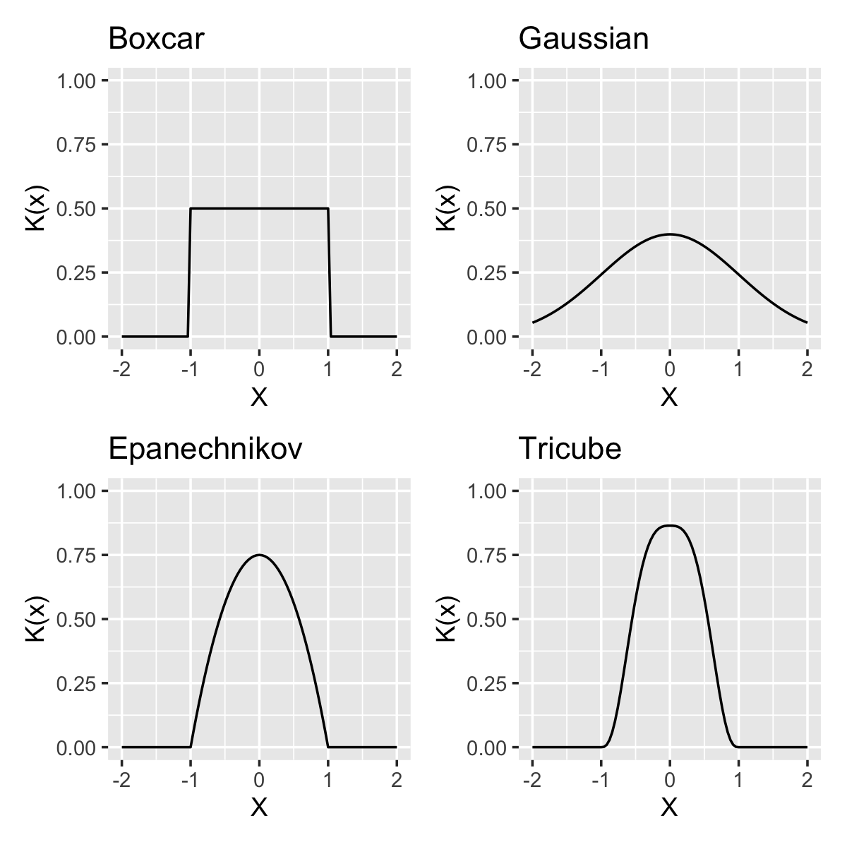
Example 20.1 (Common kernels) Often-used kernels include: \[\begin{align*} \text{boxcar} && K(x) &= \frac{1}{2} \ind(|x| \leq 1),\\ \text{Gaussian} && K(x) &= \frac{1}{\sqrt{2\pi}} e^{-x^2/2},\\ \text{Epanechnikov} && K(x) &= \frac{3}{4} \left(1 - x^2\right) \ind(|x| \leq 1)\\ \text{tricube}&& K(x) &= \frac{70}{81} \left(1- |x|^3\right)^3 \ind(|x| \leq 1) \end{align*}\] These are shown in Figure 20.1. Notice particularly that all but the Gaussian kernel are bounded, meaning their value is 0 except in a specific interval. We will see later that different kernels have different efficiencies, but that the differences are small and commonly used kernels typically produce very similar fits.

Figure 20.1: The most common kernels for kernel regression.

20.1.2 Interpreting the kernel and bandwidth

Now we can see the role of the kernel and the bandwidth together. To calculate $\hat r(x)$, the bandwidth determines which training observations are “close enough” to average over, and the kernel determines how we weight them to form the prediction. In practice, the common kernels produce very similar results, and so the bandwidth is the key tuning parameter.

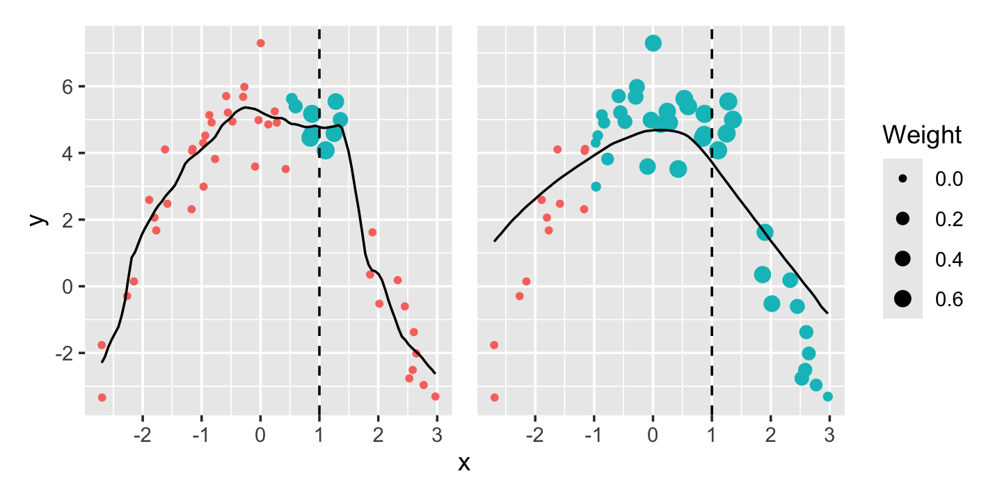
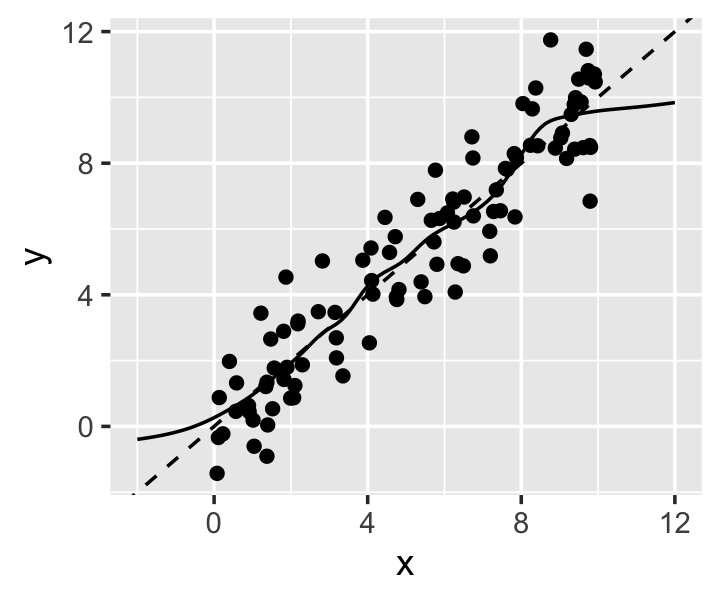
Example 20.2 (Bandwidth in kernel regression) In Figure 20.2 we can see the effect of bandwidth in a simple univariate regression. The kernel smoother (using the Epanechnikov kernel) with bandwidth $h = 1/2$ is quite jumpy, while the smoother with bandwidth $h = 2$ is much smoother. The larger-bandwidth kernel averages over more observations to make its prediction at each point, explaining the smoothness.

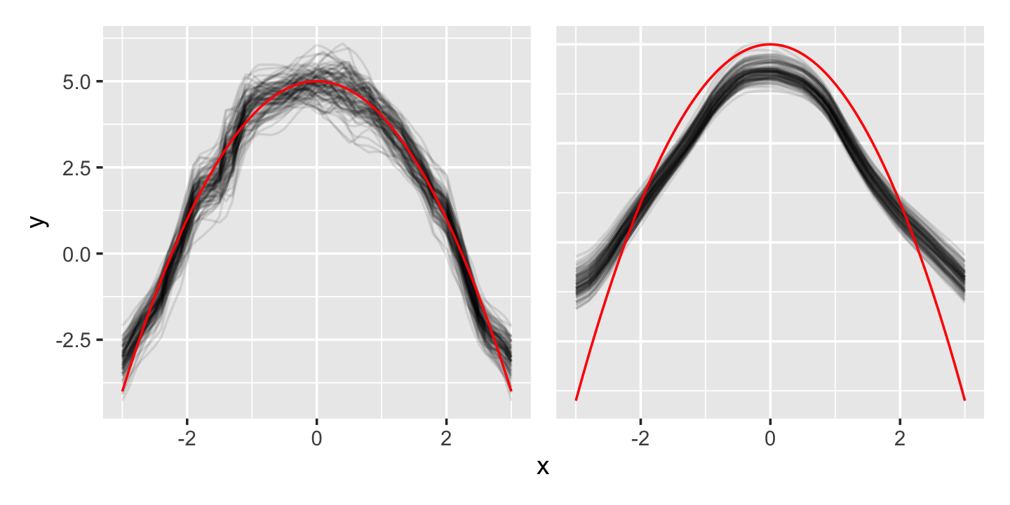
Figure 20.2: Kernel smoothers applied to data with a simple quadratic relationship, with bandwidths $h = 1/2$ (left) and $h = 2$ (right). Points are sized according to their weight for predicting at $x = 1$.

However, Figure 20.3 illustrates the tradeoff. The larger-bandwidth kernel has lower variance, but because it averages over a larger range, it tends to be biased. For instance, at $x = 0$ (the peak of the curve), it averages over points to the left and right—which are all lower than the peak, causing it to produce an average that is too low. This is a common problem with kernel smoothers, which tend to cut off the tops of peaks and fill in the bottoms of valleys.

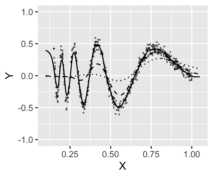
Figure 20.3: Kernel smoothers refit 100 times to new samples from the same quadratic relationship shown in Figure 20.2. At left, the smoother with $h = 1/2$ has high variance but tracks the true relationship (in red) well; at right, the smoother with $h = 2$ has much lower variance but is quite biased except around $x \pm 2$.

Example 20.3 (Kernel regression for the Doppler function) Let’s return to the Doppler function we’ve used before, most recently in Example 14.1, to see how bandwidth and kernel choices affect fits. The range of the data is between 0.15 and 1, so it is reasonable to consider smaller bandwidths. We can fit a kernel smoother using the np package. By default, it uses a Gaussian kernel, though this can be set with the ckertype argument to npreg().

library(np)
options(np.messages = FALSE) # hide its progress output

bws <- c(0.01, 0.05, 0.1)
fits <- lapply(bws, function(bw) {
  npreg(y ~ x, data = doppler_samp, bws = bw)
})

The resulting fits are shown in Figure 20.4. All the fits, even with small bandwidths, tend to “trim the peaks and fill the valleys”: at extrema, the kernel regression averages over points around the peak, which are inevitably less extreme.

Figure 20.4: Gaussian kernel fits to the Doppler function at bandwidths 0.01, 0.05, and 0.1. Notice how the fits tend to “trim the peaks”, and larger bandwidths heavily oversmooth.

20.1.3 Bandwidth selection

If our goal is to use kernel smoothing to estimate the true relationship $Y = r(X) + e$ so we can accurately predict $r(X)$, the obvious approach to select the bandwidth is cross-validation (Section 18.3). One can simply pick a range of reasonable bandwidth values, try them all, and use the value determined to be the best by cross-validation. But as the generalization error is a smooth function of the bandwidth, it can also be numerically optimized.

Example 20.4 (Bias, variance, and MSE with bandwidth) Consider the conditional generalization error (Definition 17.5), which we showed in Theorem 17.2 has a bias-variance decomposition. Let’s use simulation to obtain the bias, variance, and conditional generalization error $R(x)$ for the situation in Example 20.2, focusing on the peak at $x = 0$.

First, let’s consider what we expect. As $h$ grows, we should expect $\var(\hat r(0))$ to decrease, as it will be based on larger and larger samples (up to a maximum when the bandwidth is so large that we effectively average all the data). But we should expect $\bias(\hat r(0))$ to increase, because observations farther from $x = 0$ all have $Y$ values that are too low. There should be a sweet spot where the bias and variance sum up to the lowest value.

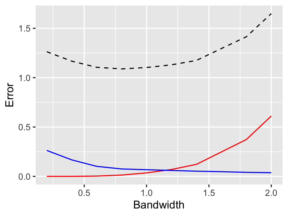
Figure 20.5: The bias-variance tradeoff in kernel regression. In red, the squared bias increases with bandwidth, while the variance (in blue) decreases. As a result, the MSE (black) has a minimum around $h = 0.8$.

Figure 20.5 shows the result, calculated by simulating 1,000 samples from the quadratic population in Example 20.2 and calculating the bias and variance of $\hat r(0)$ across the samples. The results match our expectations. By the bias-variance decomposition, $R(x)$ is the sum of the squared bias, the variance, and the irreducible error $\var(e \mid X = x)$ (which is 1 in our simulation), and this is plotted as well. There is a clear minimum around $h = 0.8$.

In short, then, Example 20.4 shows that $R(x)$ is a smooth convex function of the bandwidth $h$. If we estimate the expected generalization error with cross-validation we will observe a similar pattern, though with random noise from the cross-validation. Rather than using a grid of bandwidths and estimating the error for each, we can pick two starting bandwidths, estimate their errors, and use these to decide whether to increase or decrease the bandwidth. We then iteratively evaluate the error, determine if the bandwidth is too high or too low, and adjust again, essentially doing a numerical optimization where each function evaluation requires cross-validation.

This is how the np package automatically estimates bandwidth if you do not provide one.¹ For instance, on the data from Example 20.2:

npreg(y ~ x, data = kernel_samp)


Regression Data: 50 training points, in 1 variable(s)
                      x
Bandwidth(s): 0.2125827

Kernel Regression Estimator: Local-Constant
Bandwidth Type: Fixed

Continuous Kernel Type: Second-Order Gaussian
No. Continuous Explanatory Vars.: 1

The output reports the estimated bandwidth. Don’t be alarmed that this is smaller than the best bandwidth in Figure 20.5—the figure only plots $R(0)$, not the expected generalization error across all values of $x$.

This does, however, raise a question: If $R(x)$ is optimized by different bandwidths for different values of $x$, can we adaptively choose the bandwidth? That is, can the bandwidth vary depending on $x$ in some fashion that depends on the data?

There are indeed adaptive bandwidth selection procedures. They are very appealing for functions like the Doppler function (Example 20.3) that vary dramatically in smoothness: in smooth areas, a large bandwidth is good, but in non-smooth areas a small bandwidth allows the estimate to adapt to the local shape of the data. Typical adaptive procedures vary the bandwidth proportional to the local density of training observations, so areas with more data have smaller bandwidths and vice versa. However, use of these procedures is outside the scope of this course.

20.1.4 Discrete predictors

As we have defined them, the kernel function $K$ is appropriate for continuous real-valued predictors only. However, kernel regression can indeed be defined for categorical data as well (Li and Racine 2003). Suppose, for instance, that $X \in \{0, 1\}$. The estimator is again a weighted average of $Y$: \[ \hat r(x) = \sum_{i=1}^n \frac{K(x, x_i) Y_i}{\sum_{j=1}^n K(x, x_j)}, \] and the kernel function is quite simple: \[ K(x, x_i) \propto \begin{cases} 1 - \lambda & \text{if $x_i = x$}\\ \lambda & \text{if $x_i \neq x$}. \end{cases} \] Hence if $\lambda = 0$, we average only over cases with identical values of the discrete predictor; as we increase $\lambda$, we also average over cases with different values of the predictor.

The np package automatically implements kernels for categorical predictors and attempts to optimize $\lambda$ in the same way as it optimizes the bandwidth $h$ of continuous kernels.

20.2 Local linear and local polynomial smoothers

Kernel regression estimates are flexible and adaptable to any reasonably smoothly varying regression function, but they do suffer some important problems. Notably, they suffer a boundary effect. If the training data $(X_1, Y_1), \dots, (X_n, Y_n)$ is observed on some interval $X_i \in [a, b]$, then estimates of $\hat r(a)$ and $\hat r(b)$, and nearby points, will be biased.

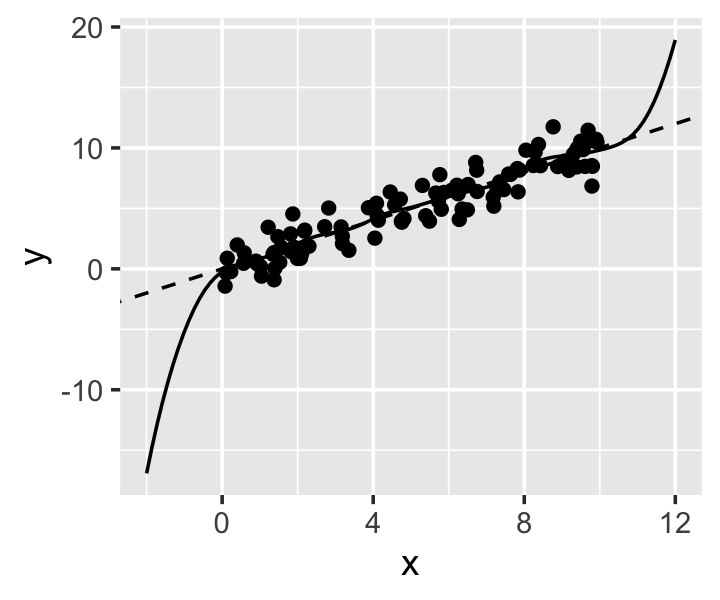
Example 20.5 (The boundary effect) As a simple example, consider a population where $X \in [0, 100]$ and its association with $Y$ is linear.

library(np)

kfit <- npreg(y ~ x, data = linear_samp, bws = 0.5)

In Figure 20.6 we see the data and the kernel fit. Outside the interval, the fit quickly becomes flat, as the kernel estimator can only average nearby points, not extrapolate. The slope begins flattening even inside the interval.

Figure 20.6: Kernel smoother fit to a linear trend, with the dashed line indicating the true population association. Notice that outside the range of the data, the predictions become flat.

The boundary effect arises because the kernel regression only takes averages. But if the ordinary kernel regression estimator uses a weighted average to estimate $\hat r(x)$, why not use a weighted regression to estimate $\hat r(x)$? Just as the weights change depending on the point we are predicting in kernel smoothing, we can solve different weighted regression problems at each point of interest. This leads to local linear regression.

Definition 20.2 (Local linear regression) The local linear regression estimator solves the weighted least-squares problem \[ \hat r(x) = \argmin_{r(x)} \sum_{i=1}^n K\left(\frac{x - x_i}{h}\right) (r(x_i) - Y_i)^2, \] where $r(x) = \beta_0 + \beta_1 x$. That is, the fit is the solution to a weighted least squares regression problem. The minimization is repeated for each value of $x$, so $\beta_0$ and $\beta_1$ are estimated locally, not globally.

Example 20.6 (Boundary effect revisited) In Example 20.5 we saw the boundary effect in kernel regression. Let’s repeat the same fit, but with a local linear fit. npreg() can do local linear regression by specifying regtype = "ll":

ll_fit <- npreg(y ~ x, data = linear_samp,
                bws = 0.5, regtype = "ll")

In Figure 20.7 we see the tradeoff we have made. Within the interval $[0, 10]$, there is no longer a boundary effect, because the local linear fit can learn the slope even when near a boundary. But outside the interval, the fit has high variance, because the slope estimated outside the boundary depends on the values of the training points closest to the boundary.

Figure 20.7: Local linear fit to a linear trend, with the dashed line indicating the true population association. Notice that outside the range of the data, the predictions can have unexpected slopes, depending on the values of training observations near the boundaries.

As with ordinary kernel smoothing, npreg() will use leave-one-out cross-validation to select a bandwidth if none is provided.

Of course, Definition 20.2 suggests we need not stop at local linear regression: provided our bandwidth is wide enough to ensure there are sufficient observations at any point $x$, we could fit any degree of polynomial, not just a line. However, the variance of these fits will grow quite high. Let’s examine the bias and variance of kernel fits in more detail.

20.3 Bias and variance of kernel smoothers

402 lec 7

We showed in Theorem 17.2 that the conditional generalization error $R(x)$ has a bias-variance tradeoff. We’ve already explored it with simulation in Example 20.4, but we can also work out the bias and variance analytically, giving rigor to back our intuition. This is also a good example of the kind of error analysis that is done for nonparametric estimation techniques in general.

If $Y = r(X) + e$ and $\hat r(x)$ is a weighted sum of $Y$s, as defined in Definition 20.1, we can Taylor-expand each of them around $X = x$. This produces sums in terms of $r(x)$ and its derivatives. Following Shalizi (2024) section 4.2 and subtracting the Taylor expansions, we can show that given a training set $\trainset$, \[ \E[\hat r(x) - r(x) \mid \trainset] = h^2 \left( \frac{r''(x)}{2} + \frac{r'(x) f'(x)}{f(x)}\right) \sigma_K^2 + o(h^2), \] where $\sigma_K^2$ is defined as in Definition 20.1 and $f(x)$ is the density of $X$. Using the same Taylor expansion, we can find the variance, \[ \var(\hat r(x) \mid \trainset) = \frac{\sigma^2 C(K)}{n h f(x)} + o\left((nh)^{-1} \right), \] where $C(K) = \int K(x)^2 \dif x$.

Several features of these should match what we’ve seen in the previous examples:

The bias increases with $r''(x)$, the curvature of the true relationship. In Example 20.3 we saw that the kernel smoothers trimmed off peaks and filled in valleys, which are exactly the areas with large second derivatives.
The bias increases with $r'(x) f'(x)$. If the density of $X$ is constant, then a sloping $r(x)$ does not cause bias; but if the density, say, increases as $X$ increases, then a local average will include more points on one side of $x$ than on the other. If $r(x)$ is sloped, this causes bias. One case when this occurs is the boundary effect demonstrated in Example 20.5.
The bias increases with the square of the bandwidth, as we might expect from Figure 20.3.
On the other hand, the variance decreases in areas with a high density $f(x)$, because the averages will be over more observations.
The variance decreases with $h$ and $n$ because, again, increasing them allows averages to be over more observations.

The same Taylor expansion procedure can be performed for local linear regression. Interestingly, in local linear regression the bias term involving $r'(x)$ is canceled out; increasing the degree of the polynomial successively cancels out higher-order bias terms. This can also reduce or eliminate boundary effects. Hastie and Loader (1993) interpret this as local linear regression adapting the kernel to the local shape of $r(x)$, and advocate for local linear regression to be preferred over basic kernel smoothers.

If we put together the bias and variance we can produce an expression for $R(x)$. Eliminating all constant terms and only considering dependence on $h$, we obtain \[ R(x) = \sigma^2 + \underbrace{O(h^4)}_{\text{bias}^2} + \underbrace{O\left((n h)^{-1} \right)}_{\text{variance}}. \] If we differentiate and set to zero, we find that the minimum of this function is at \[ h^* = O(n^{-1/5}), \] so the optimal bandwidth declines as the sample size increases. Plugging this back into $R(x)$, we find that $R(x) = O(n^{-4/5})$ when the optimal bandwidth is used.

Compare that to parametric methods. In linear regression, for instance, when the true relationship is linear the estimates are unbiased, and $\var(\hat r(x))$ is proportional to $n^{-1}$, so $R(x) = O(n^{-1})$. The nonparametric kernel smoother has risk that declines slightly more slowly as $n$ grows—but the linear model’s bias term can explode when the true relationship is not actually linear.

TODO mention Epanechnikov efficiency proof

20.4 Multivariate kernel smoothers

So far we have only considered univariate kernel smoothers, but they can be extended to multiple dimensions. One way is to use a product kernel. If there are $p$ regressors, define the product kernel \[ K_h(x - x_i) = \prod_{j=1}^p K_j\left(\frac{x_j - x_{ij}}{h_j}\right), \] and specify bandwidths for each kernel. Then perform ordinary kernel regression (or local linear regression) using this kernel. This can adapt to arbitrary shapes in multiple dimensions, making it a good choice in multivariate problems when we can’t make assumptions about the true relationship $r(x)$. When there are discrete predictors, the product kernel can include discrete kernels (Section 20.1.4).

However, it’s only a practical choice up to about $p = 7$ dimensions. Only a small part of that issue is because now $p$ bandwidths must be selected, and the number of cross validation steps grows exponentially as we consider a grid of bandwidths in $p$ dimensions. The real problem is the variance: \[ \var(\hat r(x) \mid \trainset) = O\left( \frac{1}{n h^p} \right). \] Following the same procedure as before to get the optimal bandwidth and hence the optimal $R(x)$, we find that \[ R(x) = O(n^{-4/(p + 4)}), \] compared to the $O(n^{-4/5})$ we had in one dimension.

Example 20.7 (The exponential explosion) Suppose we have $N$ observations of 1-dimensional data. We’d like to get the same generalization error in $p$ dimensions. Setting the orders of magnitude equal, \[ O(N^{-4/5}) = O(n^{-4/(p + 4)}). \] Solving for $n$, we find we need \[ O(N^{(4 + p)/5}) \] observations in $p$ dimensions to obtain the same risk. The result is plotted in Figure 20.8. For $p = 20$, we only need about $10^9$ observations to predict as accurately as we did with 100 in one dimension!

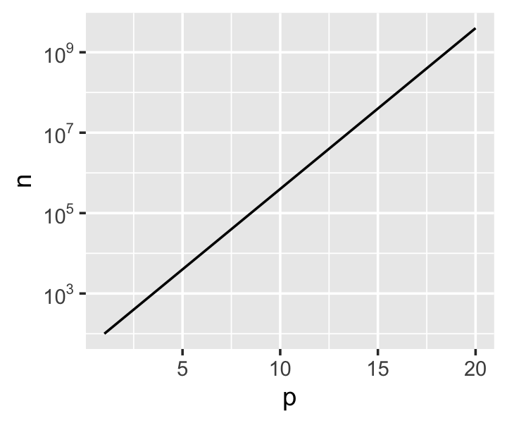
Figure 20.8: The explosion in sample size required to obtain the same prediction risk for a $p$-dimensional kernel smoother, compared to $N = 100$ observations in one dimension. Note the log scale.

This problem is the curse of dimensionality. It is one reason why additive models (Chapter 14) are so appealing: by imposing some structure on our model of $r(x)$, we have dramatically lower variance. Or, in other words, we trade bias (the possibility the relationship is not additive) for variance.

20.5 Visualizing fits

A univariate kernel regression is a smoother, and so it can easily be plotted on top of the original data in a scatterplot: plot $Y$ versus $X$ and add a smooth line at $\hat Y$ using the kernel smoother’s predictions. This is how the plots in Example 20.2 were made.

Multivariate kernel regressions, however, require more care. A kernel regression with continuous predictors $X_1$ and $X_2$ defines a two-dimensional surface. Unlike in an additive model, the two predictors are not assumed to be additive, so we can’t simply plot them separately; we’d have to make a plot in 3D showing the full surface. If we have more than two predictors, we lose the ability to visualize them.

One way to solve this is to plot slices of the surface. For instance, if we have three predictors and fit $\hat r(x_1, x_2, x_3)$, we can plot $\hat r(x_1, 0, 0)$ against $x_1$, then repeat for other values of $x_2$ and $x_3$.

20.6 Exercises

TODO 402 HW1 1, HW 5 1, exercise 17.2,

Exercise 20.1 (Origin of the kernel regression estimator) Show that the estimator $\hat r(x)$ given in Definition 20.1 is the solution to the following least-squares problem: \[ \hat r(x) = \argmin_{c} \sum_{i=1}^n K\left(\frac{x - x_i}{h}\right) (c - Y_i)^2, \] That is, the kernel regression estimate of $\hat r(x)$ minimizes the weighted sum of squared errors for predicting all $Y_i$, where the weight is given by the kernel. Observations for which $K((x-x_i)/h)$ is large are weighted higher, so the kernel regression estimate can be seen as minimizing the sum of squared errors for “nearby” observations, for a definition of “nearby” given by the kernel function.

Exercise 20.2 (Effective degrees of freedom of kernel regression) In Exercise 14.2, we showed that the effective degrees of freedom for a linear smoother can be written as $\edf(\hat r) = \trace S$, where $S$ is the smoothing matrix. Derive an expression for the effective degrees of freedom for a kernel regression, writing it in terms of the kernel, bandwidth, and observed data.

Then simulate 100 observations from the Doppler function (Figure 10.3, Example 14.1):

doppler <- function(x) {
  sqrt(x * (1 - x)) * sin(2.1 * pi / (x + 0.05))
}

doppler_pop <- population(
  x = predictor(runif, min = 0.15, max = 1),
  y = response(
    doppler(x),
    error_scale = 0.05
  )
)

doppler_samp <- doppler_pop |>
  sample_x(n = 100) |>
  sample_y()

Write R code to calculate the effective degrees of freedom for a Gaussian kernel fit to this data. Plot the edf as a function of bandwidth $h$ for $h$ from 0.1 to 1.

We fit a Gaussian kernel smoother with bandwidth 0.01 to the Doppler function in Example 20.3. Compare the fit to a polynomial fit with the same effective degrees of freedom (rounded to the nearest integer). Which performs better?

This can cause npreg() and npregbw() to be incredibly slow on large datasets. The ftol and tol parameters determine the tolerance npregbw() uses to decide when to stop optimizing the bandwidth; setting them to a larger value, such as 0.01, can make the optimization much faster at the cost of a bandwidth that isn’t precisely the best.↩︎