11 Conducting Inference
\[ \DeclareMathOperator{\E}{\mathbb{E}} \DeclareMathOperator{\R}{\mathbb{R}} \DeclareMathOperator{\RSS}{RSS} \DeclareMathOperator{\AIC}{AIC} \DeclareMathOperator{\bias}{bias} \DeclareMathOperator{\MSE}{MSE} \DeclareMathOperator{\VIF}{VIF} \DeclareMathOperator{\var}{Var} \DeclareMathOperator{\cov}{Cov} \DeclareMathOperator{\cor}{Cor} \DeclareMathOperator{\se}{se} \DeclareMathOperator{\trace}{trace} \DeclareMathOperator{\vspan}{span} \DeclareMathOperator{\proj}{proj} \newcommand{\condset}{\mathcal{Z}} \DeclareMathOperator{\cdo}{do} \newcommand{\ind}{\mathbb{I}} \newcommand{\T}{^\mathsf{T}} \newcommand{\X}{\mathbf{X}} \newcommand{\Y}{\mathbf{Y}} \newcommand{\Z}{\mathbf{Z}} \newcommand{\zerovec}{\mathbf{0}} \newcommand{\onevec}{\mathbf{1}} \newcommand{\trainset}{\mathcal{T}} \DeclareMathOperator*{\argmin}{arg\,min} \DeclareMathOperator*{\argmax}{arg\,max} \DeclareMathOperator{\SD}{SD} \newcommand{\dif}{\mathop{\mathrm{d}\!}} \newcommand{\convd}{\xrightarrow{\mathrm{D}}} \DeclareMathOperator{\logit}{logit} \newcommand{\ilogit}{\logit^{-1}} \DeclareMathOperator{\odds}{odds} \DeclareMathOperator{\dev}{Dev} \DeclareMathOperator{\sign}{sign} \DeclareMathOperator{\normal}{Normal} \DeclareMathOperator{\binomial}{Binomial} \DeclareMathOperator{\bernoulli}{Bernoulli} \DeclareMathOperator{\poisson}{Poisson} \DeclareMathOperator{\multinomial}{Multinomial} \DeclareMathOperator{\uniform}{Uniform} \DeclareMathOperator{\edf}{edf} \]
Sooner or later, everyone using regression starts asking about inference: Is the model statistically significant? Is the coefficient statistically significant? Is this model significantly better than that model? These questions are dangerous because there are, in principle, precise answers—but they are often answers to the wrong questions, and sometimes we aren’t even sure what question we’re asking.
11.1 What hypothesis do you want to test?
The first and most important thing to do when you are tempted to check for statistical significance is this: Ask what you really want to know. With fast computers, R, and thousands of packages implementing thousands of methods, we can conduct hypothesis tests as fast as we can think of them. But we must take care to ensure those tests will actually answer our questions.
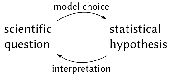
We can think of a mapping between scientific questions and statistical hypotheses (Figure 11.1). Each scientific question might be answerable with many different statistical hypotheses, depending on the data and the model we choose; but any particular statistical hypothesis might also correspond to multiple contradictory scientific questions. A statistician must be able to translate between scientific questions and statistical hypotheses, choosing the statistical hypotheses and tests that would best test the scientific question of interest.
Let’s consider a hypothetical example described by Bolles (1962):
Two groups of rats are tested for water consumption after one, the experimental group, has been subjected to a particular treatment.
| Group | 0 cc. | 1 cc. | 2 cc. | 3 cc. | 4 cc. | … | 12 cc. |
|---|---|---|---|---|---|---|---|
| Control | 15 | 3 | 2 | 0 | 0 | … | 0 |
| Treatment | 12 | 3 | 0 | 0 | 4 | … | 1 |
The data is shown in Table 11.1. The scientific question is whether the treatment changes the water consumption of the rats. But there are many statistical hypotheses that correspond to that. We could test if the mean water consumption of the two groups is different: a \(t\) test would be an obvious choice, but the data is not normally distributed, so we could use a nonparametric test like the Mann–Whitney test, or we could use a permutation test. Each has different power to detect different types of change in the mean given different distributions of data.
We could also test if the distribution of water consumption of the two groups is different. (Maybe the treatment changes the variance or skew.) We could use a \(\chi^2\) test, a Kolmogorov–Smirnov test, or some other test of distributions.
In short, for one simple situation, we could list perhaps ten different statistical procedures with a few minutes of thought. Identifying appropriate procedures—and ruling out inappropriate ones—requires understanding of the data and the question to be answered.
Once we choose a procedure, we obtain a result and need to translate it back to the scientific question. This is also not trivial, as Bolles explains:
The problem here, basically, is that the statistical rejection of the null hypothesis tells the scientist only what he was already quite sure of—the animals are not behaving randomly. The fact that the null hypothesis can be rejected with a \(p\) of \(.99\) does not give [the scientist] an assurance of \(.99\) that his particular hypothesis is true, but only that some alternative to the null hypothesis is true.1
There are other alternative scientific hypotheses that would produce the same statistical outcome. What if something is wrong with the water bottles installed in the rat cages?
But let us suppose, however, that there occurs, every once in a while, a bubble in the animal’s home-cage drinking tube, which prevents normal drinking. If this were the case, and if bubbles occur, say, 2.5% of the time, then about 50% of the time a bubble will appear in the experimental group, so [the scientist] will get just the results he got about 50% of the time.
Testing a particular scientific hypothesis, then, requires a careful choice of statistical methods, then a careful interpretation of their results. To distinguish between different scientific hypotheses that offer competing explanations, we must find some way the statistical results can distinguish between those hypotheses.
The role of the statistician is hence not simply to be a human flow-chart, following rules about which tests apply to which kind of data and spewing out \(p\) values. A good applied statistician must understand the science nearly as well as the scientist, while having a keen awareness of how statistical methods work and how their results should be interpreted. Let’s see this in action for regression.
11.2 The t test
Many useful null hypotheses can be written in terms of linear combinations of the coefficients. For example, consider a linear model with a continuous predictor \(X_1\) and a binary factor entering as a dummy-coded regressor \(X_2 \in \{0, 1\}\): \[\begin{align*} Y &= \beta_0 + \beta_1 X_1 + \beta_2 X_2 + \beta_3 X_1 X_2\\ &= {\underbrace{(\beta_0 + \beta_2 X_2)}_{\text{intercept}}} + {\underbrace{(\beta_1 + \beta_3 X_2)}_{\text{slope}}} X_1. \end{align*}\] We could think of several null hypotheses to test:
- \(\beta_2 = 0\): the two factor levels have identical intercepts
- \(\beta_3 = 0\): the two factor levels have identical slopes
- \(\beta_1 = c\): the slope when \(X_2 = 0\) is some value \(c\) predicted by a theory we are testing
- \(\beta_1 + \beta_3 = 0\): when \(X_2 = 1\), there is no association between \(X_1\) and \(Y\)
- \(\beta_2 = \beta_3 = 0\): the two factor levels have identical relationships between \(X_1\) and \(Y\)
There are undoubtedly others, and the number of plausible hypotheses only multiplies as we add predictors to the model.
The first four of these hypotheses can be written in the form \[ H_0: a\T \beta = c, \] for some chosen \(a \in \R^p\) and a scalar \(c\). (The last hypothesis will have to wait for Section 11.3.) To test these, we can use Theorem 5.6, which holds that under the null hypothesis, \[ \frac{a\T \hat \beta - c}{S \sqrt{a\T (\X\T \X)^{-1} a}} \sim t_{n - p}. \] Because the test statistic has a \(t\) distribution, this is often known as the \(t\) test (though there are many other tests with \(t\)-distributed statistics). We can alternately write the test statistic as \[ t = \frac{a\T \hat \beta - c}{\sqrt{a\T \hat \Sigma a}}, \] where \(\hat \Sigma\) is our estimate of \(\var(\hat \beta)\). This form will be particularly convenient for calculation in R. Often we test hypotheses where \(c = 0\)—so often that R conducts this test for every coefficient by default.
Example 11.1 (Palmer Penguins test) Let’s return to the Palmer Penguins data introduced in Example 7.3. This time we will look only at gentoo penguins, and our research question is whether the slope of the relationship between flipper length and bill length depends on body mass.
library(palmerpenguins)
library(dplyr)

gentoo <- penguins |>
  filter(species == "Gentoo")

gentoo_fit <- lm(bill_length_mm ~ flipper_length_mm *
                   body_mass_g,
data = gentoo)gentoo_fit.
| Characteristic | Beta | 95% CI | p-value |
|---|---|---|---|
| (Intercept) | 152 | 3.5, 301 | 0.045 |
| flipper_length_mm | -0.55 | -1.2, 0.15 | 0.12 |
| body_mass_g | -0.03 | -0.06, 0.00 | 0.058 |
| flipper_length_mm * body_mass_g | 0.00 | 0.00, 0.00 | 0.039 |
| Abbreviation: CI = Confidence Interval | |||
As shown in Table 11.2, this model has 4 coefficients, and the interaction slope is the fourth. We construct our vector a and produce a \(t\) statistic:
beta_hats <- coef(gentoo_fit)
a <- c(0, 0, 0, 1)

t_stat <- sum(a * beta_hats) /
  sqrt(a %*% vcov(gentoo_fit) %*% a)[1,1]
t_stat
[1] 2.090275(We have indexed the denominator with [1,1] because otherwise the result would be a \(1 \times 1\) matrix, which is inconvenient.) This result matches exactly the \(t\) statistic that R calculates in the model summary output (or in tidy(gentoo_fit)), and we can obtain the \(p\) value using pt(). The df.residual() generic function (Section 6.1) computes the residual degrees of freedom for fitted models, which is equal to \(n - p\), so we do not need to count:
p_value <- pt(t_stat, df.residual(gentoo_fit),
              lower.tail = FALSE)
p_value
[1] 0.01936113This is a one-tailed test: it calculates the probability \(\Pr(t_{n-p} \geq t)\). This would be appropriate if we had prespecified the alternative hypothesis \[ H_A : \beta_3 \geq 0, \] with some prior knowledge that we expected the coefficient to be positive, rather than the more generic alternative hypothesis \[ H_A : \beta_3 \neq 0. \] This would be appropriate if we had no specific expectation about the direction of the effect, and matches what R calculates by default. Because the \(t\) distribution is symmetric, we can calculate the corresponding \(p\) value by multiplying by two:
p_value * 2[1] 0.03872226To report this result in text, we would say that the slope of the relationship between gentoo penguin flipper length and bill length appears to be associated with body mass, \(t(119) = 2.09\), \(p = 0.0387\).
11.3 The F test for nested models
The \(F\) test allows us to test more general null hypotheses of the form \[ H_0: A \beta = c, \] where \(A \in \R^{q \times p}\) and \(c \in \R^q\). An important special case is the null hypothesis that several coefficients are simultaneously zero: the null hypothesis \[ H_0: \begin{pmatrix} 0 & 1 & 0 & 0 \\ 0 & 0 & 0 & 1 \end{pmatrix} \begin{pmatrix} \beta_1 \\ \beta_2 \\ \beta_3 \\ \beta_4 \end{pmatrix} = \begin{pmatrix} 0 \\ 0 \end{pmatrix} \] is equivalent to \(H_0: \beta_2 = \beta_4 = 0\). This type of null hypothesis is frequently used when testing the null that, say, a relationship is linear rather than quadratic or cubic; or the null that a continuous predictor’s relationship with the response is identical regardless of the level of a factor predictor with several levels; or simply testing the null that several specific predictors are not associated with the response. We can interpret \(q\) as the number of parameters that are set to zero under the null. Or, more generally, we can think of the \(F\) test as comparing a full model (with \(\beta\) unconstrained) against a reduced model (with \(A \beta = c\)), and \(q\) as being the difference in the number of parameters between these two models, since \(A\) constrains \(q\) of the \(p\) parameters to be written in terms of the others.
When comparing a full model against a reduced model, this procedure is often referred to as a partial \(F\) test.
11.3.1 The classic version
To test this null, we could calculate \(A \hat \beta - c\) and reject the null when the vector is sufficiently far from the origin, perhaps by using its norm \(\|A\beta - c\|_2\). But \[ \var(A \hat \beta) = \sigma^2 A (\X\T \X)^{-1} A\T, \] so the entries of \(A \hat \beta - c\) have different variances. If an entry has high variance, a large value should give us less reason to reject the null than if it had low variance. This suggests a test statistic that normalizes by the variance, such as using the Mahalanobis distance (Definition 3.12), \[ (A \hat \beta - c)\T \var(A \hat \beta)^{-1} (A \hat \beta - c). \] This normalizes the entries and reduces the test statistic to a single scalar value. The null distribution of this statistic is unfortunately not easy to calculate, but we can show that an alternate version is both intuitive and has an easy-to-calculate null distribution.
Theorem 11.1 (Seber and Lee (2003), theorem 4.1) Let \(\hat \beta\) denote the least-squares fit and \(\hat \beta_H\) denote the fit subject to the constraint that \(A \hat \beta_H = c\), where \(A\) is a \(q \times p\) matrix. We can show that:
- \(\RSS(\hat \beta_H) - \RSS(\hat \beta) = (A \hat \beta - c)\T \left(A(\X\T\X)^{-1} A\T\right)^{-1} (A \hat \beta - c)\), so we can use the difference in RSS to measure deviation from the null value of \(\beta\). (Note that \(\var(A \hat \beta) = A \var(\hat \beta) A\T\), so this expression matches the test statistic we desired above, except for a factor of \(\sigma^2\).)
- When \(H_0\) is true and \(e \sim \normal(0, \sigma^2)\), the statistic \[ F = \frac{(\RSS(\hat \beta_H) - \RSS(\hat \beta))/q}{\RSS(\hat \beta)/(n - p)} \] has the distribution \(F \sim F_{q, n - p}\).
Proof. The details are not enlightening unless you enjoy matrix algebra; see Seber and Lee (2003), theorem 4.1.
The intuition here is that \(\RSS(\hat \beta_H) \geq \RSS(\hat \beta)\), because the restricted model’s column space is a subspace of the full model’s column space, and so the full model can fit better even when the null is true. When the null hypothesis is true, the difference in RSS (appropriately rescaled) follows an \(F\) distribution; when the null is false, \(\hat \beta\) will be a much better fit than \(\hat \beta_H\), and so the \(F\) statistic will be large and we will reject the null.
Of course, this is a statistical hypothesis test like any other, and so our ability to detect when the null is false depends on the sample size and how far \(\beta\) is from satisfying the constraint \(A \beta = c\). It also depends on assumptions: Theorem 11.1 relies on \(e \sim \normal(0, \sigma^2)\) to show that the test statistic has an \(F\) distribution under the null hypothesis. When this assumption is violated, the null distribution may be different. The \(F\) test is, however, considered to be “robust” to nonnormality, meaning that its null distribution is still approximately \(F\) even when the errors are not normal. The extent of the robustness depends on the sample distribution of \(\X\), surprisingly enough (Seber and Lee 2003, sec. 9.5).
In R, the generic function anova() can conduct \(F\) tests to compare multiple models. The method for linear models, anova.lm(), prints out a table containing the \(F\) statistic, \(p\) value, and various sums of squares that classically were useful for conducting tests.
Example 11.2 In Example 10.7, we created a population with two predictors: a continuous predictor and a binary factor (duck or goose). We fit a spline model for the continuous predictor and allowed it to interact with the factor, effectively fitting a different spline for each factor level.
We can test whether that was necessary. The null hypothesis is that the coefficients for the interaction regressors are all zero; the alternative is that at least some are not zero, and hence the spline coefficients are different for ducks and geese. We have a sample from the population in interact_data.
We fit two models, one with the interaction and one with only main effects:
library(splines)

interact_fit <- lm(y ~ ns(x1, knots = c(-2, 2)) * x2,
                   data = interact_data)
main_fit <- lm(y ~ ns(x1, knots = c(-2, 2)) + x2,
               data = interact_data)
Now we can use anova() to compare them. Multiple models can be provided as successive arguments; typically we place the null model first and order models by increasing numbers of parameters.
f_test <- anova(main_fit, interact_fit)
f_test
Analysis of Variance Table
Model 1: y ~ ns(x1, knots = c(-2, 2)) + x2
Model 2: y ~ ns(x1, knots = c(-2, 2)) * x2
Res.Df RSS Df Sum of Sq F Pr(>F)
1 95 2726.2
2 92 715.7 3 2010.5 86.147 < 2.2e-16 ***
---
Signif. codes: 0 '***' 0.001 '**' 0.01 '*' 0.05 '.' 0.1 ' ' 1Each row of the printed table corresponds to a model (so if we passed three models to anova(), we’d get three rows). Each row includes the residual degrees of freedom (\(n - p\) for that model), the residual sum of squares, and (for models past the first) the difference in degrees of freedom from the previous (\(q\)) as well as the \(F\) statistic and its \(p\) value. A sum of squares value is provided because it was commonly used in old-school ANOVA analyses, but we will not bother with it here.
In our case, we have \(F(3, 92) = 86.1\), \(p = 1.27\times 10^{-26}\). A significant result should not surprise us: the population was defined so that the relationship was flipped for ducks and for geese, as we could see in Figure 10.8, and so the null hypothesis is definitely false.
11.3.2 As a likelihood ratio test
The \(F\) test can also be considered a special case of the likelihood ratio test (LRT). If we specify the model to have normally distributed errors with constant variance, then the likelihood function is \[ L(\beta) = \prod_{i=1}^n \frac{1}{\sqrt{2 \pi \sigma^2}} \exp\left(-\frac{(Y_i - \beta\T X_i)^2}{2 \sigma^2}\right). \]
We can use this likelihood function to conduct a likelihood ratio test.
Theorem 11.2 (Wilks’s theorem for likelihood ratios) Let \(\Theta\) denote the full parameter space and \(\Theta_0\) denote the reduced parameter space under the null hypothesis, so that \(\Theta_0 \subset \Theta\). The likelihood ratio test statistic is \[ \lambda = \frac{\sup_{\beta \in \Theta_0} L(\beta)}{\sup_{\beta \in \Theta} L(\beta)} \] Under the null hypothesis, and assuming certain regularity conditions on the likelihood, \[ -2 \log \lambda \convd \chi_{q}^2 \] as \(n \to \infty\). Here \(\convd\) represents convergence in distribution and \(q\) is the difference in dimension between \(\Theta\) and \(\Theta_0\).
In the case of testing \(A \beta = c\) in a linear model, we have \[\begin{align*} \Theta &= \R^p\\ \Theta_0 &= \{\beta \in \R^p \mid A \beta = c\}. \end{align*}\] The likelihood ratio test statistic is then \[ \lambda = \frac{\sup_{\beta \in \Theta_0} L(\beta)}{\sup_{\beta \in \Theta} L(\beta)} = \frac{L(\hat \beta_H)}{L(\hat \beta)}, \] and \(q\) is the dimension of \(c\), or alternately the difference in number of parameters between the two models. The intuition is that under the null hypothesis that \(\beta \in \Theta_0\), maximizing the likelihood over the larger space \(\Theta\) may improve the likelihood some, but it should not improve a lot, just as we argued that \(\RSS(\hat \beta_H) \geq \RSS(\hat \beta)\) in the \(F\) test. And when we compute \(-2 \log \lambda\) for the model with normal errors, we will find it can be written in terms of the difference in RSS, making this comparison very apt (Exercise 11.7).
R can compare nested linear models using the likelihood ratio test. Provide the test = "Chisq" argument to anova() to get \(\chi^2\) statistics and \(p\) values based on them. However, the likelihood ratio test is not particularly useful for linear models, as the test statistic is only asymptotically \(\chi^2\), whereas the \(F\) statistic is exactly \(F\)-distributed when the model is correct and the errors are normally distributed with common variance. But the connection to the LRT is useful to us nonetheless: as we move into generalized linear models, RSS will no longer be a meaningful metric, and likelihood ratio tests will become the primary option for comparing models.
11.4 Goodness of fit
Besides testing individual null hypotheses with the \(t\) and \(F\) tests, it would be convenient to have tests or summaries that describe the goodness of an entire model. Then we would have a single value to check to know if our model is good.
The previous paragraph should make you nervous, for at least two reasons:
- If our goal is measuring something as vague as “goodness”, how can we produce a precise number? It’s like scoring the wholesomeness of a box of cereal. Can that be reduced to a number?
- Why are we in such a hurry to reduce complicated things to a single number, anyway?
But even if we arrogant statisticians can declare ourselves above such pursuits, many scientists and data analysts depend on them, so we should understand them.
11.4.1 Overall F test
The first commonly used summary is the overall \(F\) test. This is the test of Theorem 11.1, using \(c = \zerovec\) and \[ A = \begin{pmatrix} 0 & 1 & 0 & \cdots \\ 0 & 0 & 1 & \cdots \\ \vdots & & & \vdots\\ 0 & 0 & \cdots & 1 \end{pmatrix}. \] That is, it tests the null hypothesis \[ H_0: \beta_1 = \beta_2 = \dots = 0. \] Notice this does not include the intercept. In short, the overall \(F\) test is a nested \(F\) test comparing the given model to one with only an intercept.
Example 11.3 (Overall F test) In Example 11.2, we fit two models, one with an interaction and one without. R’s summary() function automatically conducts the overall \(F\) test for the model, so we can use it to test the model without the interaction:
summary(main_fit)
Call:
lm(formula = y ~ ns(x1, knots = c(-2, 2)) + x2, data = interact_data)

Residuals:
    Min      1Q  Median      3Q     Max
-11.149  -3.622  -0.348   3.657  13.128

Coefficients:
                          Estimate Std. Error t value Pr(>|t|)
(Intercept)                  0.481      1.909   0.252   0.8016
ns(x1, knots = c(-2, 2))1    2.635      2.467   1.068   0.2881
ns(x1, knots = c(-2, 2))2    6.056      4.679   1.294   0.1987
ns(x1, knots = c(-2, 2))3   -3.847      2.050  -1.876   0.0637 .
x2goose                     -8.649      1.094  -7.904 4.79e-12 ***
---
Signif. codes:  0 '***' 0.001 '**' 0.01 '*' 0.05 '.' 0.1 ' ' 1

Residual standard error: 5.357 on 95 degrees of freedom
Multiple R-squared:  0.4455,    Adjusted R-squared:  0.4221
F-statistic: 19.08 on 4 and 95 DF,  p-value: 1.522e-11
Notice the last line of the summary, which declares that we reject the null hypothesis with \(F(4, 95) = 19.08\), \(p = 1.5\times 10^{-11}\).
You will sometimes see people declare that because the overall \(F\) test is statistically significant, the model itself is “significant”. It’s not clear what that is supposed to mean. Yes, we have rejected the null that none of the regressors are associated with the response, but that does not mean this model is well-specified or even useful. Indeed, in the example above, we found that main_fit is “significant”, though in Example 11.2 we found the model is clearly inadequate when compared to one with an interaction. Evidently the model being “significant” does not make it correct.
Some journals expect an overall \(F\) test to be presented with every model, but unless you literally want to test if all the coefficients are zero, there is little reason to do one.
11.4.2 Coefficient of determination
You will also often see the coefficient of determination, \(R^2\), being presented to summarize a model fit.
Definition 11.1 (Coefficient of determination) The coefficient of determination, usually denoted \(R^2\), for a linear model is \[ R^2 = \frac{\widehat{\var}(\hat \Y)}{\widehat{\var}(\Y)} = \frac{\widehat{\var}(\Y) - \widehat{\var}(\hat e)}{\widehat{\var}(\Y)}, \] the ratio of the variance predicted by the model to the actual variance of the response.
By design, \(R^2 \in [0, 1]\), so it is often interpreted as the proportion of variance “explained” by the model. Large values presumably indicate your success in model-building, while small values presumably mean your model is wrong.
However, the astute reader will notice my use of “presumably” and assume some caveats are soon to follow. Indeed, the following examples will demonstrate them.
Example 11.4 (The pitfalls of the coefficient of determination) Consider two samples to which we fit two models. The samples are shown in Figure 11.2. In one sample, the true population relationship is linear; in the other, it is quadratic. In both, the population error variance is \(\sigma^2 = 1\).
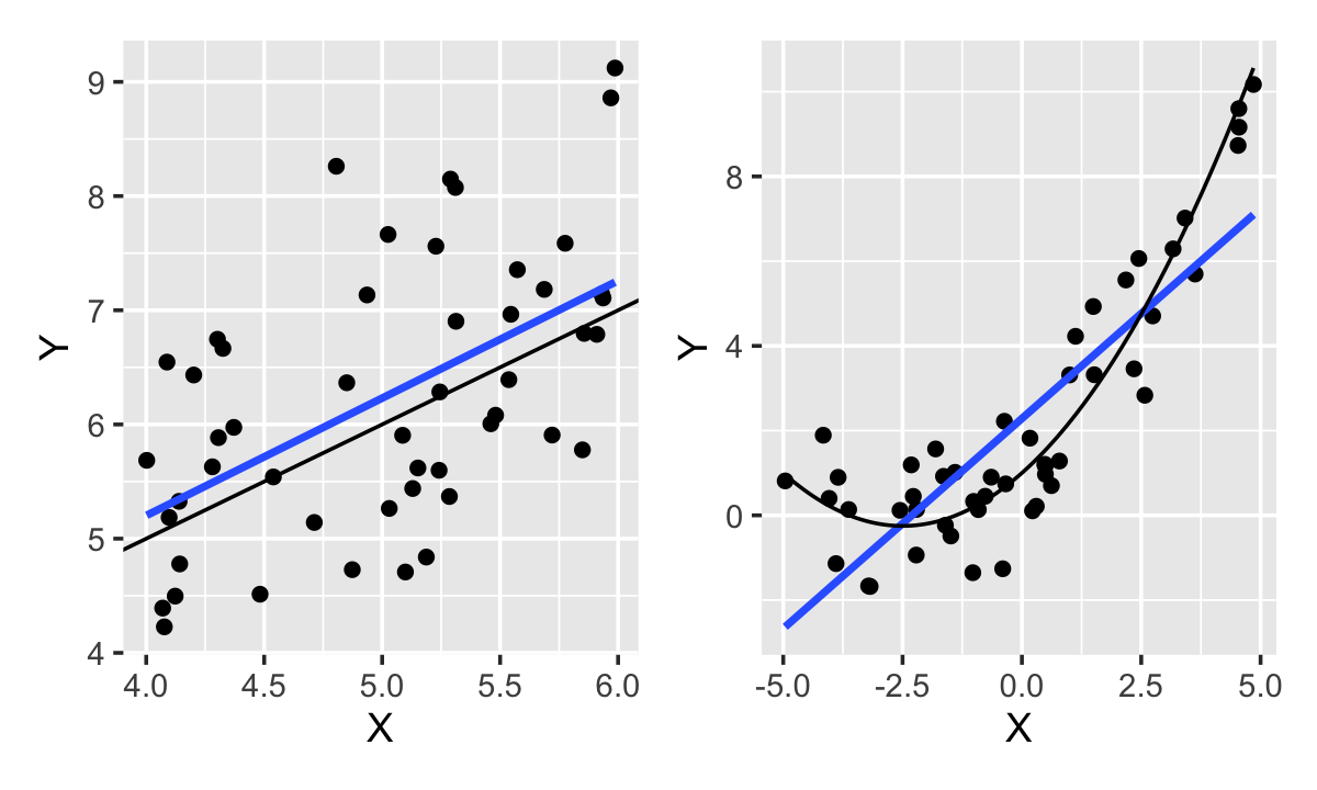
Despite the linear model being an obviously poor fit to the quadratic relationship, the fit has \(R^2 = 0.74\), while the linear fit to the true linear relationship has \(R^2 = 0.27\). Why should there be such a difference in favor of the incorrect model?
The explanation can be seen directly in Definition 11.1: \(R^2\) depends solely on the variance of the response and the variance of the residuals. The variance of the errors is identical in the two populations, so the error variance is similar; but the nonlinear relationship is observed over a larger range of \(X\) and hence has a larger variance of \(\Y\).
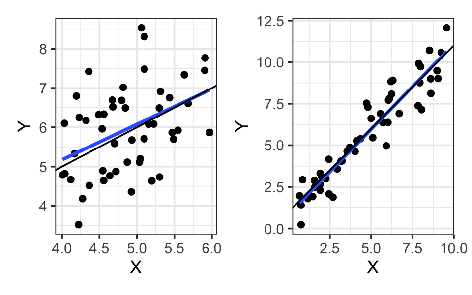
In other words, since \(R^2\) measures the proportion of variance explained, we can increase it simply by having more variance to explain, even with the same model. For instance, as shown in Figure 11.3, if we observe the linear relationship over a larger range of \(X\), we obtain \(R^2 = 0.92\). This is the same linear relationship, with the same error variance, fit to the same sample size, but now \(R^2\) is much higher!
As the example shows, \(R^2\) does not measure whether the model is correct. Nor does it measure the amount of error we expect when predicting \(Y\). Or the width of confidence intervals or prediction intervals we would make with the model. So what is it good for? To quote Shalizi (2024), section 10.3.2:
At this point, you might be wondering just what \(R^2\) is good for — what job it does that isn’t better done by other tools. The only honest answer I can give you is that I have never found a situation where it helped at all.
If you want to show a model is well-specified, use the diagnostic techniques of Chapter 9. If you want to show the parameters are precisely estimated, give their confidence intervals. If you want to show the model predicts well, we will define and measure prediction error in Chapter 16 and Chapter 17. If you want complicated questions to be answerable with a single, interpretable number, might I suggest studying a field other than statistics?
11.5 Post-selection inference
Let us suppose that, for whatever reason, you use statistical significance as a threshold, reporting only statistically significant results and removing variables whose coefficients are not significantly different from zero. Perhaps you believe this makes the model more interpretable or eliminates useless variables. What tragedy might befall you?
There are two related problems. First, reporting only significant results—only bothering to publish a paper or announce a finding if you have a significant result—leads to truth inflation. Second, once you have used significance as a filter for variables in your model, tests and confidence intervals for other variables will no longer be valid. Let’s consider each problem.
11.5.1 Truth inflation
Academia is full of publication bias: to get a result published, it must be exciting; to be exciting, it must be statistically significant. If you conduct a study to find if risk factor A is associated with bad outcome B, and you fail to find an association, most journals will reject your work because it is uninteresting. After all, there are thousands of things not associated with outcome B; what matters is identifying the things that are associated with it. Right?
But that’s not the whole story. If there’s some reason to think A is associated with B, failing to find an association gives us some information, and tells us to reconsider our theories. It also prevents other researchers from wasting time studying A, or at least suggests to them to look at A differently in future work.
And, worse, our significance filter means that, on average, published results will overestimate the size of effects. Let’s see an example to justify this.
Example 11.5 (Truth inflation) In this simulation, we are interested in the effect of \(X_1\) on \(Y\) after controlling for the confounding variable \(X_2\). The true slope is \(\beta_1 = 1/2\), and we can of course fit a regression model:
infl_pop <- population(
  x1 = predictor(rnorm, mean = 0, sd = 1),
  x2 = predictor(rnorm, mean = 0, sd = 1),
  y = response(
    4 + 0.5 * x1 - 3 * x2,
    family = gaussian(),
    error_scale = 3.0
  )
)

infl_samp <- infl_pop |>
  sample_x(n = 100) |>
  sample_y()

infl_fit <- lm(y ~ x1 + x2, data = infl_samp)
Now let’s obtain the sampling distribution of estimates for \(\beta_1\).
sdist <- sampling_distribution(infl_fit, infl_samp,
                               nsim = 1000)

x1_ests <- sdist |>
  filter(term == "x1")
The sampling distribution is shown in Figure 11.4. Notice that the distribution looks nice and normally distributed around the true mean \(\beta_1 = 1/2\), but in many of the 1000 samples, we failed to reject the null hypothesis \(H_0: \beta_1 = 0\). The mean of \(\hat \beta_1\) is unbiased for \(\beta_1\), but the mean of the significant values of \(\hat \beta_1\) is biased for \(\beta_1\).
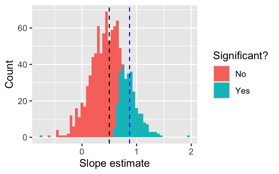
In this particular population, we only obtained statistically significant results in about 34% of the samples. This is known as the power of the test: the power is the probability of rejecting the null under a particular alternative hypothesis. Here the power depends on the sample size, the size of \(\beta_1\), the error variance \(\sigma^2\), and any correlation between \(X_1\) and \(X_2\).
Truth inflation is expected whenever significance is used as a filter for results (Ioannidis 2008). If the size of effects is as important as their presence, truth inflation is a serious problem, and misleads readers of published work into thinking effects are much stronger than they really are.
The general phenomenon of journals only publishing significant results is known as publication bias, and in recent years researchers have begun making efforts to eliminate publication bias. One idea is the registered report: researchers propose a study to answer a question of interest and submit their study design and analysis plan to a journal for review before beginning to collect data. The journal can commit to publishing the work on the grounds the methods are sound and would resolve an interesting question, before seeing results, and will publish the work even if the results are not significant.
One component to sound methods is ensuring the study has adequate power. As we saw in Example 11.5, a study with poor power will either fail to find effects that exist (perhaps falsely concluding they don’t exist) or exaggerate them. Ensuring adequate power means choosing appropriate statistical methods and collecting a sample size large enough to reliably detect an effect of interest. This can be done with simulations, as we did above, or through mathematical derivation of the sampling distribution of estimates.
11.5.2 Inference after selection
Statistical inference for parameters is based on the sampling distribution: the hypothetical distribution of estimates we would obtain if we repeatedly obtained new samples from the population. A \(p\) value, for instance, is the probability of obtaining an estimate equal to or more extreme than the one we obtained, calculated assuming the null hypothesis is true. That means that statistical inference for parameters depends on the procedure we use to generate estimates. If we use a different estimator, or perhaps include different variables in our model, we would expect the sampling distribution to be different and hence the tests and confidence intervals to be different as well.
But the procedure does not include only the final model or test we conduct. In truth inflation, we could think of the procedure as “check for significance: if insignificant, ignore this result; if significant, report the estimate”, and that procedure leads to estimates that are biased. In ordinary statistical practice, though, the procedure often involves fitting a model, checking diagnostics, changing the model, conducting some tests, changing the model again, and finally arriving at a model that is used for the main results. If we obtained a different sample from the population, every step in that procedure may have been different, and we may have chosen a different final model with very different main results. Our test or confidence interval calculation has no idea, and assumes our procedure is simply whatever final model we chose.
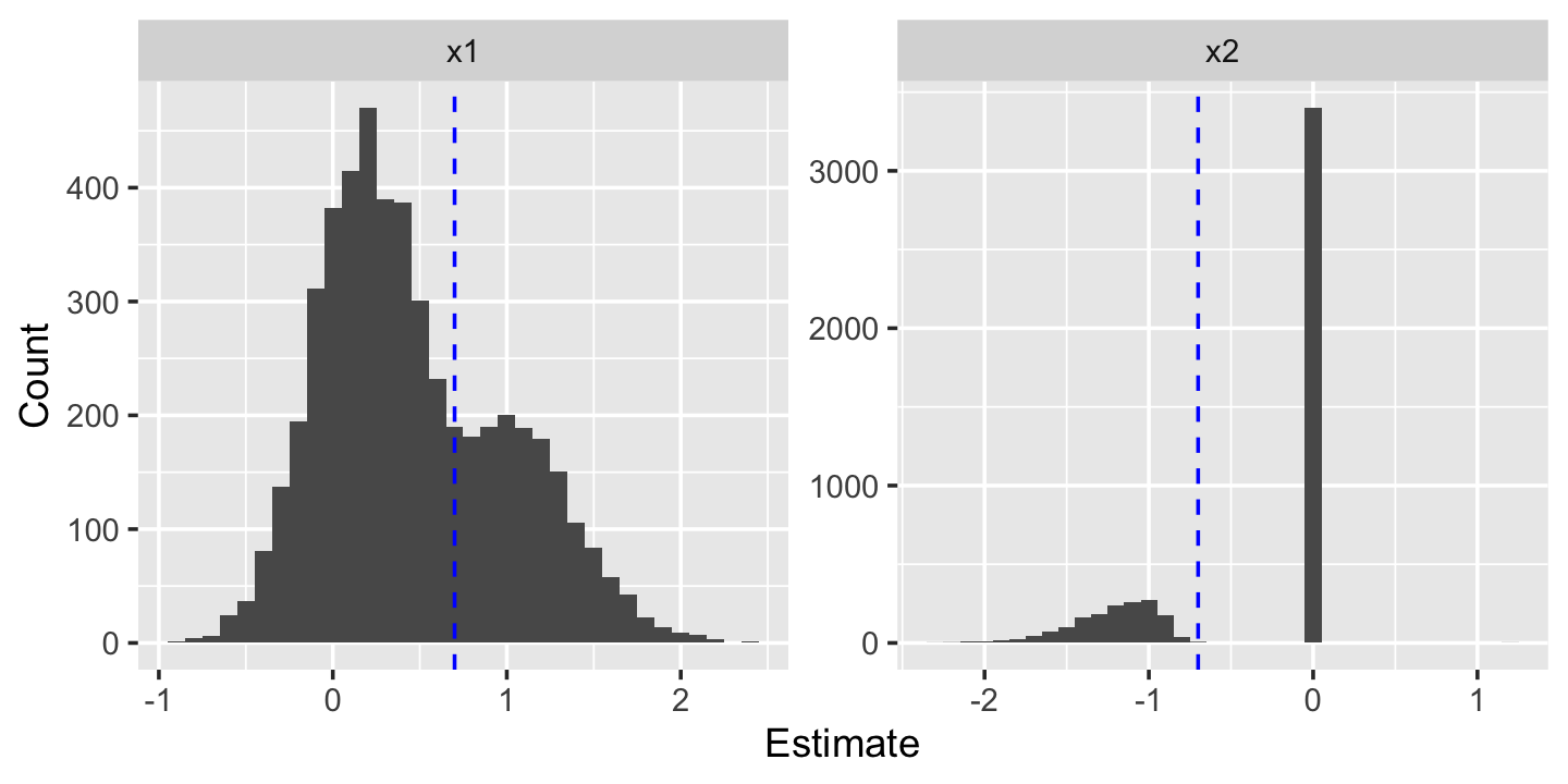
Example 11.6 (Post-selection inference) In this population, the predictors \(X_1\) and \(X_2\) are positively correlated. Imagine this represents a situation where we want to know the causal effect of \(X_1\) on \(Y\), but need to control for the confounding variable \(X_2\).
library(mvtnorm)

psi_pop <- population(
  x = predictor(rmvnorm, mean = c(0, 0),
                sigma = matrix(c(1, 3/4, 3/4, 1),
                               nrow = 2, ncol = 2)),
  y = response(
    4 + 0.7 * x1 - 0.7 * x2,
    family = gaussian(),
    error_scale = 3.0
  )
)
Let’s suppose our fitting procedure is to fit a linear model, check if the coefficient for \(X_2\) is statistically significant, and to remove it from the model if it is not. The code below simulates this procedure with 5000 draws from the population, saving all the coefficients into a data frame; in simulations where \(X_2\) was removed from the fit, we record its coefficient as \(\hat \beta_2 = 0\).
# tidy-style data frame representing \hat \beta_2 = 0
zero_x2 <- data.frame(
  term = "x2", estimate = 0, std.error = 0, statistic = 0,
  p.value = 1, conf.low = 0, conf.high = 0
)

results <- replicate(5000, {
  new_samp <- psi_pop |>
    sample_x(n = 100) |>
    sample_y()

  new_fit <- lm(y ~ x1 + x2, data = new_samp)
  coefs <- tidy(new_fit, conf.int = TRUE)

  # if x2 is not significant, refit without it
  if (coefs$p.value[coefs$term == "x2"] > 0.05) {
    new_fit <- lm(y ~ x1, data = new_samp)
    coefs <- tidy(new_fit, conf.int = TRUE)

    # add a row to indicate x2 has coefficient 0
    coefs <- rbind(coefs, zero_x2)
  }
  coefs
}, simplify = FALSE)

# combine the many data frames into a single data frame
results <- bind_rows(results)
Figure 11.5 shows the sampling distribution of the estimates from this procedure. Notice the bias in \(\hat \beta_2\): when \(X_2\) is included in the model, most of the time \(\hat \beta_2 < -1\), which is biased compared to the true value \(\beta_2 = -0.7\). Notice also that the distribution of \(\hat \beta_1\) is oddly skewed and perhaps bimodal. This non-normality will cause confidence intervals to under-cover and the skew will result in biased estimates of \(\beta_1\), as you will show in Exercise 11.9.
In short: All the inference procedures in this chapter are not valid for post-selection inference, meaning inference conducted after we use some process to select our model and the variables we include in it. There are a few ways to deal with this problem:
- Pretend it doesn’t happen. This is the most common approach, though not necessarily the wisest.
- Treat the initial study as a pilot or exploratory study, and confirm the results by collecting additional data and fitting the final model to that new dataset.
- Split your data into two pieces. Conduct your exploratory data analysis and model selection on one piece, finalize it, and then run it fresh on the untouched data. Report those results, significant or not. This is known as sample splitting.
- Use a test procedure specifically designed to account for the selection process. Valid post-selection inference was a hot research area very recently (i.e., around 2010–2020), and some useful procedures have been developed (Kuchibhotla et al. 2022). However, as Kuchibhotla et al. (2022) note, “there are significant challenges to implementation even in relatively simple linear regression problems with popular variable selection procedures”, and in general it is quite difficult to develop procedures that account for all the ways statisticians might adjust their model based on the data.
The challenge of post-selection inference emphasizes the importance of having specific scientific hypotheses to test, and converting these to specific statistical hypotheses. When our question is vague, many similar models might be suitable, and many different tests or estimates might be useful, the statistician enters a garden of forking paths (Gelman and Loken 2014): the specific methods chosen might depend heavily on the exploratory data analysis, diagnostics, and favorite procedures of the statistician. Given a different sample from the same population, the statistician might have made very different choices and picked a very different model.
The best illustration of this problem might be the “Many Analysts, One Data Set” experiment, which recruited research teams to answer a research question and compare their results:
Twenty-nine teams involving 61 analysts used the same data set to address the same research question: whether soccer referees are more likely to give red cards to dark-skin-toned players than to light-skin-toned players. Analytic approaches varied widely across the teams, and the estimated effect sizes ranged from 0.89 to 2.93 (\(\text{Mdn} = 1.31\)) in odds-ratio units. Twenty teams (69%) found a statistically significant positive effect, and 9 teams (31%) did not observe a significant relationship. Overall, the 29 different analyses used 21 unique combinations of covariates. (Silberzahn et al. 2018)
There is no statistical way to fix this problem. Data analysis requires careful thought and judgment. Humility is key: we must do the best analysis we can given the data we can collect, always being aware of the choices we make and how they may affect the results.
11.6 Statistical power
In the previous section, we defined the power of a test as the probability of rejecting the null hypothesis under a specific alternative hypothesis. Let’s define that more precisely, and explore the implications of having low power.
Definition 11.2 (Power of a test) Consider testing a null hypothesis \(H_0: \theta = \theta_0\). The test calculates a test statistic \(T\) from the observed data and rejects the null hypothesis if \(T \in R\), where \(R\) the rejection region. The power of the test under the alternative \(H_A: \theta = \theta_A\) is \[ \Pr(T \in R \mid \theta = \theta_A). \]
For example, consider a \(t\) test for a coefficient, as described in Section 11.2. We often test the null hypothesis \(H_0: \beta_j = 0\), forming a \(t\) statistic and rejecting the null if \(|t| \geq t_{n - p}^{1 - \alpha/2}\). This defines the rejection region \(R\). The power of this test hence depends on the data, the sample size, and, crucially, the true slope \(\beta_j\). It is easier to detect a difference if the sample size is large or the true slope is very different from zero; it is hard to detect a small effect in a small sample.
Example 11.7 (Power of the t test for a coefficient) If the power of a test depends on both the sample size and the effect size, we can consider the power as a bivariate function of these and make a plot of this function. Let’s do this for a univariate regression problem: there is only one predictor and we want to test whether its association with \(Y\) is nonzero. To calculate the power, we must be able to derive the distribution of the test statistic under the alternative hypothesis \(H_A: \beta_1 = \delta\), where \(\delta\) is the nonzero effect size. Fortunately, this can be done analytically for the standard \(t\) test. The test statistic for this the null \(H_0: \beta_1 = 0\) is \[ t = \frac{\hat \beta_1}{\sqrt{\widehat{\var}(\hat \beta_1)}} = \frac{\frac{\hat \beta_1 - \delta}{\sqrt{\var(\hat \beta_1)}} + \frac{\delta}{\sqrt{\var(\hat \beta_1)}}}{\sqrt{\widehat{\var}(\hat \beta_1) / \var(\hat \beta_1)}}, \] which looks needlessly complicated but puts the statistic into a useful form. Under the alternative \(H_A\), this is a standard normal (\(\hat \beta_1\) minus its mean, divided by its standard deviation) plus a constant, divided by something related to a \(\chi^2\) random variable (similar to Theorem 5.3). This is the definition of the noncentral \(t\) distribution with noncentrality parameter \(\delta/\sqrt{\var(\hat \beta_1)}\) and \(n-p\) degrees of freedom.
To calculate the power, then, we calculate the critical value for the \(t\) test of \(H_0\). Then we calculate the probability under \(H_A\) (using the noncentral \(t\) distribution) of obtaining a value equal to or more extreme than the critical value, which is the probability we would reject the null when the alternative is true.
Let’s consider a range of sample sizes and a range of slopes. We can use expand.grid() to make a data frame giving all the combinations of values:
setups <- expand.grid(n = seq(10, 150, by = 10),
                      slope = seq(0.5, 3, by = 0.1))
To calculate the power at each configuration, we’ll calculate the critical value, then use the noncentral \(t\)’s distribution function to obtain the power. To calculate the noncentrality parameter requires \(\var(\hat \beta_1)\), which is inversely proportional to \(n\) (Exercise 5.4). We will set \(\sigma^2\) so that \(\var(\hat \beta_1) = 1\) when \(n = 100\).
setups$power <- NA
for (row in seq_len(nrow(setups))) {
n <- setups$n[row]
# 1 - alpha/2 quantile of t(n - p) distribution
critical_value <- qt(1 - 0.05/2, df = n - 2)
effect_size <- setups$slope[row] / sqrt(100 / n)
lower_tail_prob <- pt(-critical_value, df = n - 2,
ncp = effect_size)
upper_tail_prob <- pt(critical_value, df = n - 2,
ncp = effect_size, lower.tail = FALSE)
setups$power[row] <- lower_tail_prob + upper_tail_prob
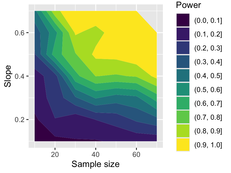
}The power is shown in Figure 11.6. We see that for slopes of about 1 when \(n = 50\), we have very little power—less than a 10% chance of obtaining a significant result. As the slopes and sample sizes increase, the power grows.
Power is an important consideration for any study. If we are conducting an experiment or collecting data ourselves, it’s important to first consider: what size effect would be interesting or important, and how much data would be required to reliably detect that effect? It would be wasteful to collect data when we would not have the power to detect any reasonable effect size. Sadly, however, power is often neglected. One review of randomized controlled trials published in top medical journals from 1975–1990 found that only 36% of the trials had at least 80% power to detect a 50% difference between treatment and control groups (Moher et al. 1994). A 50% difference seems huge! Patients recover 50% faster, or have 50% lower side effect rates, or whatever—and yet the majority of trials would have less than 80% power to detect such a huge difference. Similar problems have been found in psychology, neuroscience, and other scientific fields (Button et al. 2013; Sedlmeier and Gigerenzer 1989).
In principle, power can be calculated in advance of a study. If we know the analysis we will use and the size of effect we are looking for, we can calculate or simulate the power as a function of sample size. However, to do so requires some information we may not know: the error variance \(\sigma^2\), for example, or the correlation between different predictors, or the exact association between confounding variables and our predictor of interest. We might have to make reasonable guesses, or try different values and calculate the power to understand the range of possibilities. We also have to decide what power we want. Often 80% power is used as a desirable threshold, just like \(\alpha = 0.05\) is often used in hypothesis testing, but there’s no particular reason 80% is special. The choice depends on the importance of the question, the difficulty of obtaining sufficient data, and the cost of reaching the wrong conclusion.
Power also reminds us that if a test is not statistically significant, that does not mean there is no effect! In Figure 11.6, there are many combinations of \(\beta_1\) and sample size where the power is less than 50%. If we failed to reject the null, however, it would be incorrect to say there is no effect. We do not have enough data to reject the hypothesis that \(\beta_1 = 0\), but our data is also consistent with nonzero values of \(\beta_1\).
Finally, power reminds us of the reverse: a statistically significant result does not mean the effect is large or important. If we have a particularly large sample size, we may have adequate power to detect a very, very small effect, and we might reject the null hypothesis for a minuscule slope or association. We must be careful not to let “statistically significant” be interpreted as “significant” or “important”, and to always put our results in context by interpreting the size of the effects.
11.7 Hypothesis tests are not for model selection
You will often see scientists and statisticians use \(F\) tests (and similar tests) for model selection. By “model selection” they generally mean “choosing the correct model” or “choosing which variables should be included in the model.” They might fit several candidate models of increasing complexity, conduct several \(F\) tests, and arrive at a “final” model that is “better” on the basis of \(F\) test results. In one common version, researchers delete “insignificant” variables on the grounds they do not contribute to the model, meaning the \(F\) test for the null hypothesis that their coefficients are zero fails to reject the null.
But what is “better”? What specific goal are we trying to achieve? Consider two options:
- We are trying to test the causal relationship between certain predictors and the response. If so, we should choose variables following the principles of Chapter 2. If they are not significantly associated with the response, that does not mean they are not confounders: we may not have power to detect the relationship, but it can still bias the causal effect of interest.
- We are trying to predict the response as accurately as possible, and worry that adding too many variables will cause it to have high variance. But hypothesis tests do not measure or optimize the prediction error. We should use the error estimation and model selection methods described in Chapter 16 and Chapter 17 instead.
In neither case is it useful to delete “insignificant” variables using \(F\) tests.
The usual argument for reducing the number of variables is parsimony: the general principle that it’s better for scientific theories to be as simple as possible. A model with dozens of variables is not parsimonious, so we must remove some.
But informal model selection procedures are not guaranteed to select the “correct” variables, for any definition of correct. They are, however, guaranteed to cause post-selection inference and truth inflation problems, and make your methods more difficult to understand. If you feel the need to delete variables, consider what your goals really are, and choose a more appropriate procedure to achieve them.
11.8 Do you really need to test a hypothesis?
If a statistically significant result does not mean the effect is important, and if a non-significant result does not mean there is no effect, we need some way to describe how large the effect is. That is the job of an effect size estimate and a confidence interval. Whenever possible, hypothesis tests should be accompanied with effect sizes and confidence intervals, so the reader understands what the test result could mean.
Consider the Palmer Penguins data again (Example 7.3). We were interested in the association between flipper length (the predictor) and bill length (the response), both measured in millimeters. Suppose there was only one penguin species, so our model was \[ Y = \beta_0 + \beta_1 X + e, \] and we wanted to test \(H_0: \beta_1 = 0\). We could use a \(t\) test for the coefficient (Section 11.2). The effect size of interest is the true slope \(\beta_1\). Consider four possibilities:
- \(p < 0.05\), and the confidence interval is \([1.2, 4.8]\). We reject the null hypothesis and conclude that each millimeter of flipper length is associated with a bill that is longer by 1.2 to 4.8 millimeters, on average.
- \(p < 0.05\), and the confidence interval is \([0.0017, 0.0052]\). We reject the null hypothesis and conclude that each millimeter of flipper length is associated with a bill that is longer by less than the thickness of a single human hair. The result may be significant, but the association is tiny.
- \(p > 0.05\), and the confidence interval is \([-0.0012, 0.0004]\). We fail to reject the null, and if any association does exist, it is very small.
- \(p > 0.05\), and the confidence interval is \([-10.4, 14.2]\). We fail to reject the null, but the data would be consistent with a millimeter of flipper length being associated with a 14 millimeter longer bill, or a 10 millimeter shorter bill, or anything in between. We would need a larger dataset to narrow down the options with a smaller confidence interval.
Each of these possibilities yields very different conclusions. A statistically significant result might represent a meaningful effect or a trivially small one; an insignificant result might imply the effect is zero or nearly zero, or it might imply the effect could be anything and we simply don’t have enough data. Again, whenever possible, report the effect size and a confidence interval, and focus your interpretation on them, not on the \(p\)-value.
11.9 Further reading
The problem of connecting scientific hypotheses to testable statistical hypotheses is broader that we can cover here. Generally the problem is worst when the scientific hypothesis is least specific: it is much easier to test a theory of physics that predicts an experimental result to ten decimal places than it is to test, say, a psychological theory about human behavior. It is very difficult to make a precise and testable claim about human behavior to ten decimal places, and theories are often vague enough that, at best, they can predict that an association will be nonzero. And it is hard to distinguish between competing theories when they make vague and overlapping predictions. The interested reader should pursue outside reading on this subject.
The psychologist Paul Meehl spent much of his career pointing out these problems, and his work is an excellent summary of the challenge in testing scientific theories with data (Meehl 1990). More recently, there has been substantial debate in academic psychology about the role of more precise and formal theories (including mathematical theories) in psychology. Eronen and Bringmann (2021) give a good summary of why less precise theories make it hard to make progress, while Muthukrishna and Henrich (2019) advocated for specific and testable theories, giving the example of one theory from evolutionary biology that does make specific mathematically testable predictions.
These issues are not specific to psychology—any field making theories about how the world works is affected—but a great deal of discussion has taken place in psychology. More broadly, it is worth reading Platt (1964) on the scientific method, “strong inference”, and how to use data and experiments to improve our understanding of reality.
Exercises
Exercise 11.1 (Muscle cars) In Chapter 6, we used the mtcars data built into R to demonstrate how to fit linear models. Let’s use it again to demonstrate \(t\) tests. Fit a model for the relationship between horsepower and time to drive a quarter mile (qsec ~ hp). Conduct a \(t\) test for whether the slope is 0, and report your results. Do the test once manually, as in Example 11.1, and verify it matches the statistic and \(p\) value reported by summary().
Exercise 11.2 (Weisberg (2014), problem 6.4) The alr4 package contains the data frame UN11 giving national economic, health, and welfare statistics for 210 countries and territories. The data is from 2009–2011 and categorizes countries and territories into three groups: OECD countries (those in the Organization for Economic Co-operation and Development, a club for mostly richer countries), African nations, and “other”.
The lifeExpF variable gives the life expectancy of women, in years. The ppgdp variable gives the per-capita gross domestic product (in US dollars).
Suppose an economist predicts that life-expectancy should be proportional to log(ppgdp), but the intercepts may vary by group because of other national factors.
Fit a model to predict
lifeExpFas a function oflog(ppgdp), allowing the intercept to vary by group. Show a table or plot summarizing the model fit.Conduct a \(t\) test to determine if the OECD and “other” countries have equal intercepts. Report your result in a sentence or two.
Conduct a \(t\) test to determine if the “other” and African countries have equal intercepts. Report your result in a sentence or two.
Exercise 11.3 (Moral rebels) In 2008, a study claimed to show that “moral rebels”—those who refuse to conform with behavior they think is morally wrong—are appreciated by outsiders but not by those involved with the activity they rebel against, and hypothesized that this was because those involved feel threatened: accepting the moral rebel would mean admitting their own behavior is wrong, and it is easier to condemn the rebel than to admit you were wrong. The study involved several experiments in which participants completed tasks while others (planted by the experimenters) refused to do so on moral grounds (Monin et al. 2008).
We are interested in experiment 4, which tested the hypothesis that self-affirmation—doing some task that makes you feel good about yourself—would make it easier to accept a moral rebel. The full experiment and dataset (from a later replication) is described at https://cmustatistics.github.io/data-repository/psychology/moral-rebels.html. Read the description of the experiment and the hypothesis being tested.
Draw a causal diagram connecting the observable variables in the experiment. What path or paths are the scientists interested in?
Describe a statistical hypothesis you could test using the data provided, and say how it would connect to the scientific question. Specifically:
- Specify a model (or models) and a test (or tests) you could conduct.
- Write out the null hypotheses you would test mathematically, in terms of the parameters and their null values.
- Indicate how the test results would support or oppose the scientific hypothesis (for example, if a particular difference is positive, it supports the hypothesis, but if it’s zero or negative it does not).
There may be several plausible hypotheses you could tests from different models, but you only need to pick one and explain it.
Hint: The dataset includes several possible outcome variables; the original study combined
Other.Work,Other.Friend, andOther.Respectinto a combined score by averaging them. You could choose to do this as well, to simplify the situation; but that might have consequences for your scientific interpretation.Suppose your tests are statistically significant. Make up three plausible scientific explanations that do not involve self-affirmation making it easier to accept a moral rebel. (By “scientific explanation” I mean an explanation for why people who did the self-affirmation task accepted rebels at a different rate.)
Download the dataset and conduct EDA. Present plots summarizing the data and illustrating the relationships in question.
Fit the models you chose to fit in part 2. Present your results with a suitable table, figure, or explanatory paragraph. Comment on what this means for the scientific question, given your statistical results.
Comment on what other tests or experiments would be necessary to rule out the other explanations you devised in part 3.
Exercise 11.4 (Can you use an \(F\) test?) For each question below, determine if it can be answered by comparing two nested linear models with a partial \(F\) test. If it can’t be, explain why not. If it can be, give the model formulas (in R syntax) to fit the two models. You do not need to actually fit the models.
- In the Palmer Penguins data (Example 7.3), consider the relationship between bill length and flipper length. Do Adelie penguins have a steeper slope for this relationship than gentoo penguins?
- In the dihydrogen monoxide example (Example 7.4), does the efficacy of treatment depend on whether the patient has antibodies for dihydrogen monoxide?
- In Nelder’s dose-response example (Example 7.5), suppose we measure the variables
response,dosage, andadjuvant_dosage. Does the adjuvant cause no response on its own, or do higher doses of adjuvant actually appear to affect the response?
Exercise 11.5 (Life expectancy) Return to the data in Exercise 11.2. Conduct an \(F\) test for the equality of intercepts between all three groups. Write the null and alternative hypotheses explicitly in terms of the model coefficients being tested, and write out the \(F\) test result in a sentence or two.
Exercise 11.6 (College Scorecard) The United States Department of Education maintains a College Scorecard website, tracking thousands of colleges and universities across the US, their demographics, graduation rates, tuition costs, student loans, and much more, including average salaries after graduation. An extract of the data from 2023 is available at https://cmustatistics.github.io/data-repository/daily-life/college-scorecard.html.
First, review the data. Note that missing data is marked with the string PrivacySuppressed. You should filter out colleges with missing data in the columns we will use for this problem. (The na.strings option to read.csv() can be used to read these values as NA, and then the complete.cases function can easily remove all cases with missing values. But only remove cases with missing values in the variables you’re using, otherwise you’ll remove most of the dataset.)
Make a scatterplot of the relationship between
SATMTMID(median SAT math scores) andMD_EARN_WNE_P10(median earnings of students 10 years after entry). Look for outliers. Find these outliers in the data and look up their name (INSTNM). Can you explain the outliers?Ignore the outliers for the rest of this problem.
Suppose we want to model the relationship between median earnings and SAT math scores. Fit an ordinary linear model, plot the residuals, and look at diagnostics. Does the relationship seem to be linear? Are there any problems with the fit, and do the outliers seem to be affecting it substantially?
Consider some possible nonlinear fits. First, fit a second-order polynomial (using
poly()inlm()). Is there evidence this helps the model fit over a line? What about a third-order polynomial? Use partial \(F\) tests (withanova()) to compare the models, and explain your conclusions.
Exercise 11.7 (Equivalence of LRT and F test) Show that for a linear model with normally distributed errors, the likelihood ratio test statistic \(-2 \log \lambda\) from Section 11.3.2 can be written in terms of the difference in RSS between full and reduced model. Is this equivalent to the partial \(F\) statistic? Assume \(\sigma^2\) is estimated using the full model.
Exercise 11.8 (Coefficient of determination and correlation) Show that in the simple regression model \[ Y = \beta_0 + \beta_1 X + e, \] the coefficient of determination \(R^2\) (Definition 11.1) is the square of the sample correlation between \(X\) and \(Y\).
Exercise 11.9 (Post-selection inference) Run the code from Example 11.6 and examine the results data frame.
- Estimate the coverage of confidence intervals for \(\beta_1\). Recall that the coverage is the fraction of confidence intervals that include the true value, \(\beta_1 = 0.7\). The nominal coverage is 95%; how far off are these confidence intervals from having correct coverage?
- Estimate the power of the test used to determine whether to include \(X_2\) in the model, by calculating the percentage of times it was included.
- Estimate the bias of the estimates of \(\hat \beta_1\). How biased is this procedure?
- In a real-world problem, we would not know the true correlation between \(X_1\) and \(X_2\) or their true association with \(Y\). If you are interested in the causal effect of \(X_1\) and have some reason to believe \(X_2\) is a confounder, what does this imply about the procedure you should use? Should you be removing insignificant confounders?
You must be careful not to interpret Bolles as meaning that rejecting the null with \(p < 0.01\) means that \(\Pr(H_A \text{ is true}) > 0.99\). Bolles is using “assurance” informally here. See Reinhart (2015), chapter 4, for the mistake of interpreting \(p\) values as probabilities of the null hypothesis being true.↩︎