seeds <- read.csv("data/seeds.csv")13 Other Response Distributions
\[ \DeclareMathOperator{\E}{\mathbb{E}} \DeclareMathOperator{\R}{\mathbb{R}} \DeclareMathOperator{\RSS}{RSS} \DeclareMathOperator{\AIC}{AIC} \DeclareMathOperator{\bias}{bias} \DeclareMathOperator{\MSE}{MSE} \DeclareMathOperator{\VIF}{VIF} \DeclareMathOperator{\var}{Var} \DeclareMathOperator{\cov}{Cov} \DeclareMathOperator{\cor}{Cor} \DeclareMathOperator{\se}{se} \DeclareMathOperator{\trace}{trace} \DeclareMathOperator{\vspan}{span} \DeclareMathOperator{\proj}{proj} \newcommand{\condset}{\mathcal{Z}} \DeclareMathOperator{\cdo}{do} \newcommand{\ind}{\mathbb{I}} \newcommand{\T}{^\mathsf{T}} \newcommand{\X}{\mathbf{X}} \newcommand{\Y}{\mathbf{Y}} \newcommand{\Z}{\mathbf{Z}} \newcommand{\zerovec}{\mathbf{0}} \newcommand{\onevec}{\mathbf{1}} \newcommand{\trainset}{\mathcal{T}} \DeclareMathOperator*{\argmin}{arg\,min} \DeclareMathOperator*{\argmax}{arg\,max} \DeclareMathOperator{\SD}{SD} \newcommand{\dif}{\mathop{\mathrm{d}\!}} \newcommand{\convd}{\xrightarrow{\mathrm{D}}} \DeclareMathOperator{\logit}{logit} \newcommand{\ilogit}{\logit^{-1}} \DeclareMathOperator{\odds}{odds} \DeclareMathOperator{\dev}{Dev} \DeclareMathOperator{\sign}{sign} \DeclareMathOperator{\normal}{Normal} \DeclareMathOperator{\binomial}{Binomial} \DeclareMathOperator{\bernoulli}{Bernoulli} \DeclareMathOperator{\poisson}{Poisson} \DeclareMathOperator{\multinomial}{Multinomial} \DeclareMathOperator{\uniform}{Uniform} \DeclareMathOperator{\edf}{edf} \]
Logistic regression is just one type of generalized linear model (GLM). Again, generalized linear models have two parts:
- The systematic part describes the relationship between the mean of \(Y\) and some function of \(\beta\T X\)
- The random part describes the distribution of \(Y\) around that mean.
Specifically, the systematic part is of the form \[ g(\E[Y \mid X = x]) = \beta\T x, \] where \(g\) is known as the link function. For example, in logistic regression, \(g\) was the logit function. The random part gives the distribution of \(Y\) as an exponential dispersion family distribution, as we will describe below—for now it suffices to know that we will only use certain distributions, not any arbitrary distribution.
We use a generalized linear model when \(Y\) takes on limited values or is known to be non-normal. We used logistic regression, for instance, for problems where \(Y \in \{0, 1\}\); in other settings, when \(Y \in \{0, 1, 2, \dots\}\), it might be reasonable to model \(Y\) has being Poisson-distributed, and we can use a GLM for that too.
13.1 Exponential families
Generalized linear models work when the random part, the response distribution, is an exponential family distribution, which we will define momentarily. The exponential family is not magic, and there is nothing stopping you from creating a new kind of model that uses a different distribution; the key is that exponential family distributions all share useful properties that help us fit GLMs and do inference.
Definition 13.1 (Exponential dispersion family) The exponential dispersion family consists of distributions whose probability density or probability mass function can be written in the form \[ f(x; \theta, \phi) = \exp\left(\frac{x \theta - b(\theta)}{a(\phi)} + c(x, \phi)\right), \] where \(\phi\) is the dispersion parameter and \(\theta\) is the natural parameter. Different distributions in the family can be created by choosing different functions for \(a\), \(b\), and \(c\).
There are many ways to rearrange and rewrite this definition that you may encounter in other books and sources. We will follow Agresti (2015), section 4.1, for our formulation.
Many useful distributions are exponential family distributions.
Example 13.1 (Normal distribution) If \(X \sim \normal(\mu, \sigma^2)\), it has the probability density function \[\begin{align*} f(x; \mu, \sigma^2) &= \frac{1}{\sqrt{2 \pi} \sigma} \exp\left(- \frac{(x - \mu)^2}{2 \sigma^2} \right)\\ &= \exp\left( \frac{x \mu - \mu^2 / 2}{\sigma^2} - \frac{\log(2 \pi \sigma^2)}{2} - \frac{x^2}{2 \sigma^2}\right). \end{align*}\] This is an exponential dispersion family distribution with natural parameter \(\theta = \mu\), dispersion parameter \(\phi = \sigma^2\), and \[\begin{align*} a(\phi) &= \sigma^2 \\ b(\theta) &= \frac{\mu^2}{2} \\ c(x, \phi) &= - \frac{\log(2 \pi \sigma^2)}{2} - \frac{x^2}{2 \sigma^2}. \end{align*}\] Notice this definition treats \(\sigma^2\) as fixed and known, and only \(\mu\) is a parameter to be estimated.
Example 13.2 (Poisson distribution) If \(X \sim \poisson(\lambda)\), it has the probability mass function \[\begin{align*} f(x; \lambda) &= \frac{e^{-\lambda} \lambda^x}{x!}\\ &= \exp\left(x \log (\lambda) - \lambda - \log(x!)\right). \end{align*}\] This is an exponential dispersion family distribution with natural parameter \(\theta = \log \lambda\), dispersion parameter \(\phi = 1\), and \[\begin{align*} a(\phi) &= 1 \\ b(\theta) &= \exp(\theta) = \lambda \\ c(x, \phi) &= - \log(x!). \end{align*}\]
Example 13.3 (Binomial distribution) If \(nX \sim \binomial(n, p)\), so that \(x\) is the sample proportion of successes and \(n\) is fixed, \(X\) has the probability mass function \[\begin{align*} f(x; n, p) &= \binom{n}{nx} p^{nx} (1 - p)^{n - nx} \\ &= \exp\left( \frac{x \theta - \log(1 + \exp(\theta))}{1 / n} + \log \binom{n}{nx} \right). \end{align*}\] This is an exponential dispersion family distribution with natural parameter \(\theta = \logit(p) = \log(p/ (1 - p))\), dispersion parameter \(\phi = 1/n\), and \[\begin{align*} a(\phi) &= 1 / n\\ b(\theta) &= \log(1 + \exp(\theta))\\ c(x, \phi) &= \log \binom{n}{nx}. \end{align*}\]
The above examples cover three of the most common distributions we will use, but there are many other examples of exponential dispersion family distributions, such as the gamma distribution (Exercise 13.1). Exponential family distributions share some useful properties that we will exploit when defining generalized linear models.
Theorem 13.1 (Exponential family properties) If \(X\) is drawn from an exponential dispersion family distribution, as defined in Definition 13.1, then: \[\begin{align*} \E[X] &= b'(\theta)\\ \var(X) &= b''(\theta) a(\phi). \end{align*}\]
Proof. We can write the log-likelihood function \(\ell(\theta)\) as \[ \ell(\theta) = \frac{x \theta - b(\theta)}{a(\phi)} + c(x, \phi). \] Consequently, \[\begin{align*} \ell'(\theta) &= \frac{x - b'(\theta)}{a(\phi)} \\ \ell''(\theta) &= - \frac{b''(\theta)}{a(\phi)}, \end{align*}\] where the primes represent derivatives with respect to \(\theta\).
Two properties of the maximized log-likelihood are (Schervish 1995, 112–13) \[\begin{align*} \E[\ell'(\theta)] &= 0, & \E[\ell'(\theta)^2] &= - \E[\ell''(\theta)]. \end{align*}\] From the first property, we have that \[\begin{align*} \E[\ell'(\theta)] &= \frac{\E[X - b'(\theta)]}{a(\phi)} \\ 0 &= \frac{\E[X - b'(\theta)]}{a(\phi)} \\ b'(\theta) &= \E[X], \end{align*}\] as desired.
From the second property, we have that \[\begin{align*} \E[l'(\theta)^2] &= -\E[l''(\theta)]\\ \E\left[\frac{(X - b'(\theta))^2}{a(\phi)^2} \right] &= -\E\left[- \frac{b''(\theta)}{a(\phi)} \right]\\ \E[(X - b'(\theta))^2] &= a(\phi) \E[b''(\theta)]. \end{align*}\] Because \(b'(\theta) = \E[X]\), the left-hand side is simply \(\var(X)\). Because \(b''(\theta)\) is not random, we can further simplify to \[ \var(X) = a(\phi) b''(\theta), \] as desired.
Now we must connect the exponential family distribution to the covariates to produce a regression model. This is the job of the link function \(g\). In principle, since we are modeling \(g(\E[Y \mid X = x]) = \beta\T x\), we can use any link function such that \(g^{-1}(x)\) is always in the domain of \(Y\) for the chosen response distribution. But certain link functions will make the mathematics easier.
Definition 13.2 (Canonical link function) If \(Y\) is drawn from an exponential dispersion family distribution with natural parameter \(\theta\), the canonical link for that distribution is the function such that \[ g(\E[Y \mid X = x]) = \theta. \] Because GLMs model \(g(\E[Y \mid X = x]) = \beta\T x\), in a GLM using the canonical link, \(\beta\T x = \theta\). The covariates directly model the response distribution’s natural parameter.
For example, if \(nX \sim \binomial(n, p)\) as in Example 13.3, then \(\E[X] = p\) and \(\theta = \logit(p)\), and so \(g(p) = \logit(p)\) is the canonical link function. Table 13.1 gives the canonical link function for the most commonly used exponential family distributions.
| Distribution | Range | Canonical link | Mean |
|---|---|---|---|
| \(Y \sim \normal(\mu, \sigma^2)\) | \((-\infty, \infty)\) | \(g(x) = x\) | \(\beta\T X\) |
| \(Y \sim \bernoulli(p)\) | \(\{0, 1\}\) | \(g(x) = \logit(x)\) | \(\ilogit(\beta\T X)\) |
| \(nY \sim \binomial(n, p)\) | \([0, 1]\) | \(g(x) = \logit(x)\) | \(\ilogit(\beta\T X)\) |
| \(Y \sim \poisson(\lambda)\) | \(\{0, 1, 2, \dots\}\) | \(g(x) = \log(x)\) | \(\exp(\beta\T X)\) |
13.2 Fitting a generalized linear model
Just as with logistic regression, we will fit generalized linear models using maximum likelihood. Each observation \(i\) may have a different mean, so we will write \(\theta_i\) for the natural parameter. The log-likelihood function is \[\begin{align*} \ell(\beta) &= \sum_{i=1}^n \log f(y_i; \theta_i, \phi) \\ &= \frac{y_i \theta_i - b(\theta_i)}{a(\phi)} + c(y_i, \phi). \end{align*}\] When we use the canonical link function, \(\theta_i = \beta\T x_i\), so this becomes \[ \ell(\beta) = \sum_{i=1}^n \frac{y_i \beta\T x_i - b(\beta\T x_i)}{a(\phi)} + c(y_i, \phi). \]
To maximize the likelihood, we take its gradient with respect to \(\beta\): \[\begin{align*} D\ell(\beta) &= \sum_{i=1}^n \frac{y_i x_i - b'(\beta\T x_i) x_i}{a(\phi)} \\ &= \sum_{i=1}^n \frac{(y_i - b'(\beta\T x_i)) x_i}{a(\phi)} \\ &= \frac{\X\T(\Y - P)}{a(\phi)}, \end{align*}\] where \(P \in \R^n\) is a vector with entries \(P_i = b'(\beta\T x_i)\). If we set this equal to zero to try to find a maximum, we will unfortunately find that there is no analytical solution. We can instead proceed numerically, again using Newton’s method (Definition 12.2). We will need the Hessian of the log-likelihood: \[ D^2 \ell(\beta) = - \X\T W \X, \] where \(W\) is a diagonal matrix with entries \[ W_{ii} = b''(\beta\T x_i). \] This should look familiar: in Section 12.2.1, the Newton–Raphson procedure for fitting logistic regression had very similar gradients and Hessians, and could be done by a sequence of iteratively reweighted least squares problems. The same is true here, by exactly the same procedure. The estimator has the same properties and allows the same inference procedures as described in Section 12.4 and Section 12.6.
The gradient and Hessian above were derived for the canonical link function, but similar expressions can be obtained for other link functions with extra bookkeeping to keep track of the link function’s derivative. When not using the canonical link, Fisher scoring (which uses \(\E[D^2 \ell(\theta)]\) instead of \(D^2 \ell(\theta)\) for each update) no longer is the same as IRLS, and Fisher scoring is preferable because it provides the correct Fisher information matrix on the final step.
This simplicity of optimization illustrates why we chose to consider only exponential dispersion family distributions: the same procedure can fit a GLM using any of them, merely by knowing the functions \(a\) and \(b\) characterizing the distribution. This will also help us prove properties and describe inference procedures that work on the entire class of models, instead of having to derive new results for each model we use.
Let’s now consider some common kinds of GLMs and how they can be used.
13.3 Binomial outcomes
The binomial distribution is a common response distribution whenever outcomes are binary, or whenever we count a certain binary outcome out of a total number of trials. As one special case, \(\binomial(1, p) = \bernoulli(p)\), so logistic regression is just a GLM with a binomially distributed response with \(n = 1\). (This is why we set family = binomial() when calling glm().) Often we refer to the binary outcomes as “successes” and “failures”, so a binomial random variable is the number of successes out of a fixed number of trials.
The binomial distribution is suitable when there is a fixed and known total number of trials. The probability mass function shown in Example 13.3, and hence the likelihood function, depends on the number of trial \(n\), so it must be known. Each observation hence consists of a number of successes and a total number of trials; the number of trials may differ between observations. With \(n\) fixed, the model relates the success probability \(p\) to the predictors, so the interpretation of coefficients is much like the interpretation in logistic regression (Section 12.3).
For a binomial response, the logit is the canonical link function, though sometimes the standard normal CDF is used; this is called the “probit” link. The two link functions are very similar in shape, so they tend to produce very similar fitted models, though the logit link has the advantage of easier interpretation in terms of log-odds, odds, and odds-ratios. With either link function, the model is \[ n_i Y_i \mid X_i = x_i \sim \binomial\left(n_i, g^{-1}(\beta\T x_i)\right), \] where \(g\) is the link function. The sample proportion \(Y_i\) should hence be proportional to \(g^{-1}(\beta\T x_i)\).
In R, a binomial response variable can be provided as a binary factor (as we saw in logistic regression) or, for \(n > 1\), a two-column matrix providing the number of successes and the number of failures.
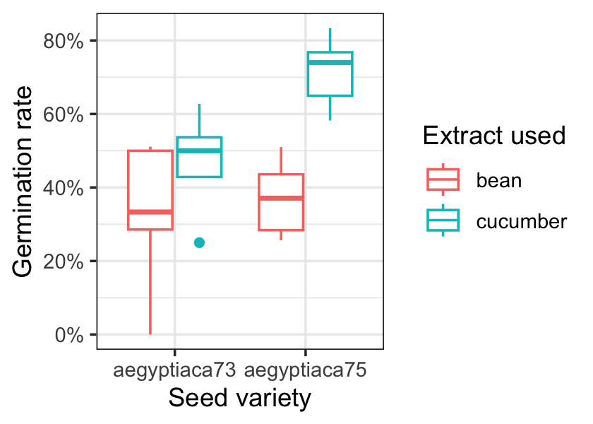
Example 13.4 (Seed germination) Orobanche is a genus of small parasitic plants that do no photosynthesis of their own, instead attaching their roots to nearby plants to steal water and nutrients from them. Whitney (1978) was interested in understanding the behavior of seeds of several Orobanche species: The seeds only germinate when in the presence of materials from the roots of their host species. As some of the hosts are commercial crops (such as beans and cucumbers), it would be valuable to figure out when the seeds germinate and identify compounds that might prevent them from doing so.
This data comes from a factorial experiment on Orobanche aegyptiaca seeds (Crowder 1978), which can parasitize many crops. There are two varieties of seed (collected from infected cucumbers in either 1973 or 1975), and two types of extract the seeds can be treated with (bean and cucumber). The goal of the experiment was to figure out which combination of seed and extract leads to the highest rate of germination of the seeds.1
A factorial design means the researchers tested each possible combination in (nearly) equal numbers. Each row of the data set seeds.csv represents one group of seeds grown together, getting the same seeds and extract; we have the total number of seeds in that group and the number that successfully germinated.
Figure 13.1 shows the germination rate for each combination of seed and extract. It looks like 1975 seeds with cucumber extract have the highest germination rate, but we can use a model to explore the differences in more detail.
For each row \(i\) of data, let \(n_i\) be the number of seeds tested, \(Y_i\) the number that germinated, and \(X_i\) be the vector of covariates (seed and extract type). A binomial model would make sense here, and if we use the default link function, our model would be \[ Y_i \sim \binomial(n_i, \ilogit(\beta\T X_i)). \]
Let’s explore whether the effect of extract is identical for both seed varieties, or if instead the extract’s effect differs by seed type. To do so, we fit two models, one with an interaction and one without.
seed_fit_1 <- glm(cbind(germinated, total - germinated) ~
                    extract + seed,
                  data = seeds, family = binomial())
seed_fit_2 <- glm(cbind(germinated, total - germinated) ~
                    extract * seed,
                  data = seeds, family = binomial())
We can again use a deviance test (Theorem 12.4) to determine if the interaction is statistically significant here.
seed_test <- anova(seed_fit_1, seed_fit_2, test = "Chisq")
seed_test
Analysis of Deviance Table
Model 1: cbind(germinated, total - germinated) ~ extract + seed
Model 2: cbind(germinated, total - germinated) ~ extract * seed
Resid. Df Resid. Dev Df Deviance Pr(>Chi)
1 18 39.686
2 17 33.278 1 6.4081 0.01136 *
---
Signif. codes: 0 '***' 0.001 '**' 0.01 '*' 0.05 '.' 0.1 ' ' 1We conclude that the extract effect differs by seed type, \(\chi^2(1) = 6.41\), \(p = 0.011\).
The coefficients of the interaction model are shown in Table 13.2. If we were interested obtaining the probability of germination for each seed/extract combination, and hence find the best-performing combination, these coefficients are inconvenient: we’d have to manually calculate the predicted probabilities and their standard errors. Instead we can make the predictions and let R do the work:
| Characteristic | OR | 95% CI | p-value |
|---|---|---|---|
| extract | |||
| bean | — | — | |
| cucumber | 1.72 | 1.05, 2.81 | 0.031 |
| seed | |||
| aegyptiaca73 | — | — | |
| aegyptiaca75 | 0.86 | 0.56, 1.34 | 0.5 |
| extract * seed | |||
| cucumber * aegyptiaca75 | 2.18 | 1.19, 3.97 | 0.011 |
| Abbreviations: CI = Confidence Interval, OR = Odds Ratio | |||
xs <- expand.grid(seed = c("aegyptiaca75", "aegyptiaca73"),
                  extract = c("bean", "cucumber"))
predictions <- predict(seed_fit_2, newdata = xs,
                       type = "response", se.fit = TRUE)
The predictions are shown in Table 13.3. We see that the ’75 seeds with cucumber extract have the highest predicted probability. These standard errors are calculated by calculating the standard error of \(\hat \beta\T x\), then using the delta method to transform this to a standard error for the probability; to obtain confidence intervals, we could calculate confidence intervals on the link scale and then transform them to the probability scale.
| Seed | Extract | Germination rate | SE |
|---|---|---|---|
| aegyptiaca75 | bean | 0.364 | 0.029 |
| aegyptiaca73 | bean | 0.398 | 0.044 |
| aegyptiaca75 | cucumber | 0.681 | 0.027 |
| aegyptiaca73 | cucumber | 0.532 | 0.042 |
13.4 Poisson regression
If a certain event occurs with a fixed rate, and the events are independent (so that the occurrence of one event does not make another more or less likely), then the count of events over a fixed period of time will be Poisson-distributed. This makes Poisson GLMs well-suited for response variables that are counts.
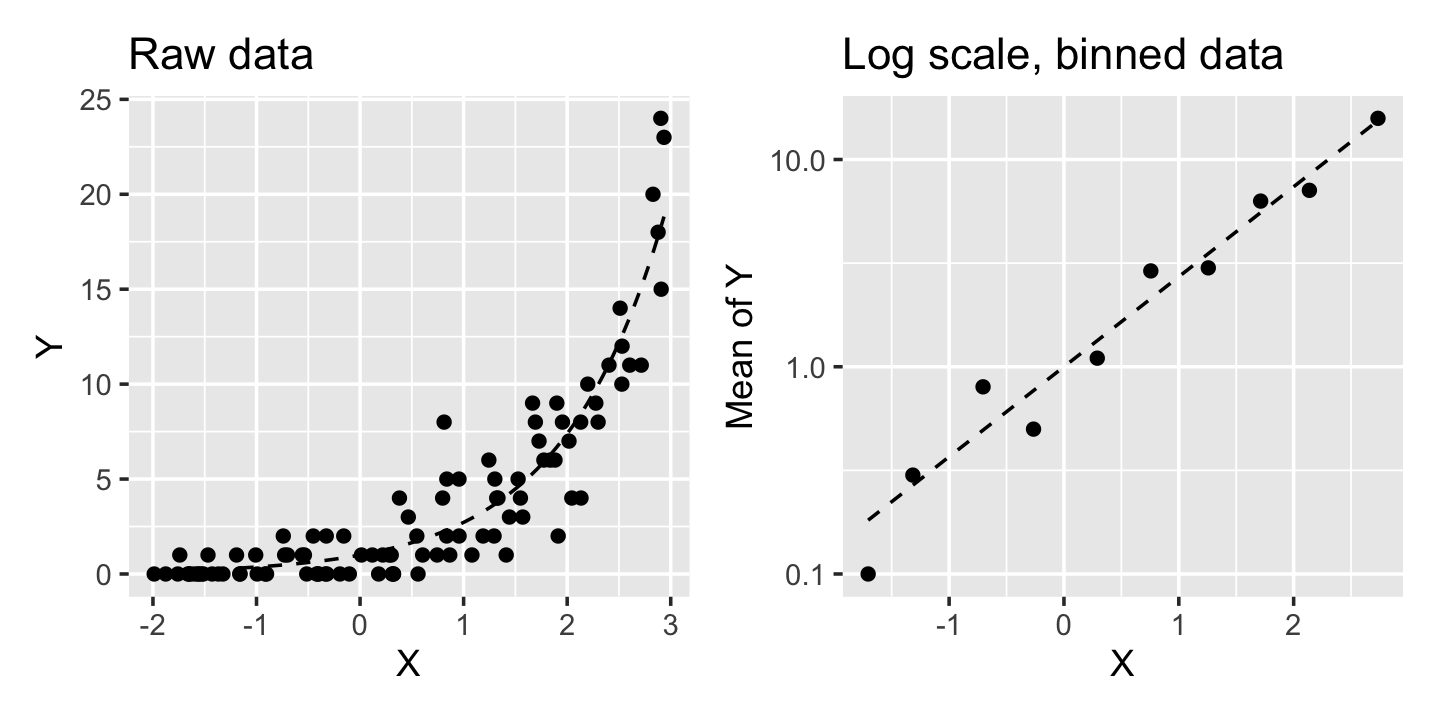
As shown in Table 13.1, the canonical link for a Poisson GLM is the log link. That is, a canonical Poisson GLM assumes the relationship \[ \log(\E[Y \mid X = x]) = \beta\T x, \] or equivalently, \[ \E[Y \mid X = x] = \exp(\beta\T x). \] And because the variance of a Poisson-distributed random variable increases with its mean, the variance of \(Y\) depends on \(X\). Figure 13.2 illustrates the relationship for a Poisson GLM where \(\log(\E[Y \mid X = x]) = x\). Notice that \(Y\) only takes on integer values and has a nonlinear relationship with \(X\), but when we group \(Y\) into bins and take the average in each bin, the log of that average is linearly related to \(X\).
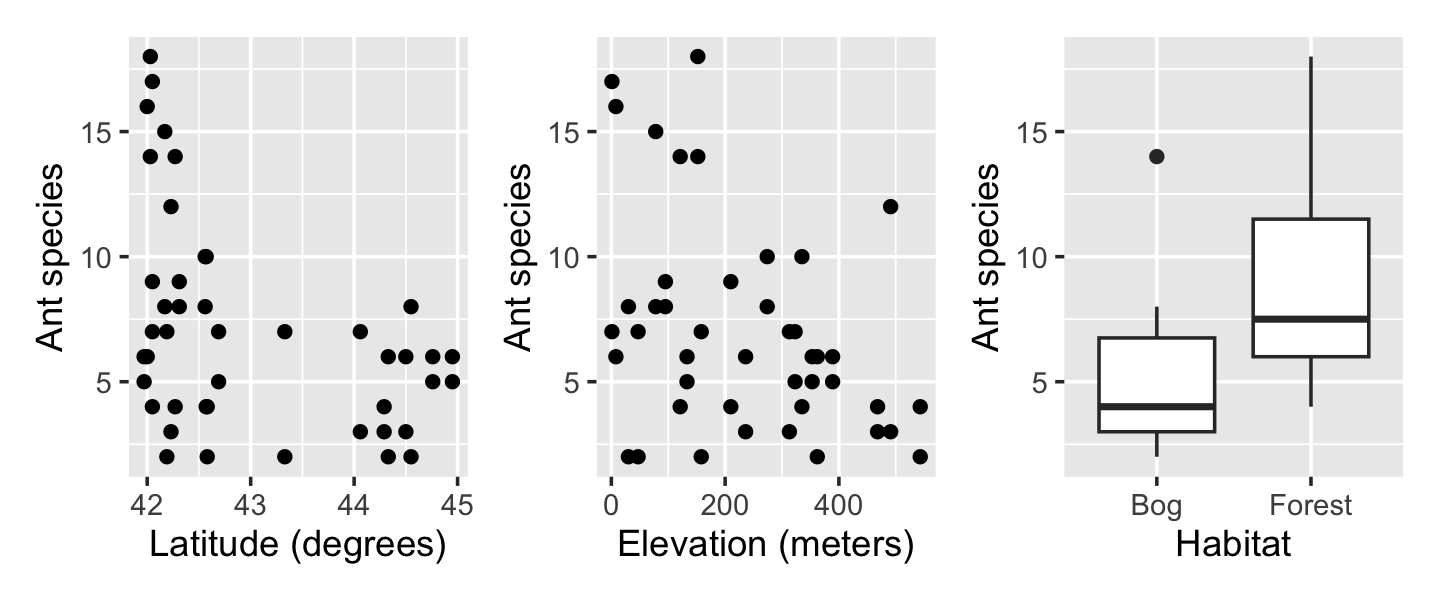
Example 13.5 (Ant diversity) Gotelli and Ellison (2002) studied the diversity of ant species in New England. Understanding why biodiversity varies by area is an important problem in ecology, and ants are a good test case because they are important in ecosystems and because their diversity varies so much across regions.
To gather their data, they sampled 64-square-meter areas in various bogs and forests in New England, counting the number of ant species in each area. Along with the count, they recorded the habitat (forest or bog), its latitude (in degrees), and its elevation (meters above sea level). The data is provided in ants.csv.
ants <- read.csv("data/ants.csv")Exploratory plots in Figure 13.3 demonstrate that the covariates appear to be correlated with the response. As the response is counts, a Poisson regression appears to be appropriate. We can fit one using glm().
ants_fit <- glm(Srich ~ Latitude + Elevation + Habitat,
                data = ants, family = poisson())
Coefficients from the fit are shown in Table 13.4. Just as we must be careful with logistic regression coefficients because they are in terms of log-odds, here we must be careful because of the log link. Formally, the model is \[ Y \mid X = x \sim \poisson(\exp(\beta_1 + \beta_1 x_1 + \beta_2 x_2 + \beta_3 x_3)), \] and so a one-unit increase in \(X_1\) is not associated with a change in \(Y\) of \(\beta_1\). The coefficients are on the link scale—the scale of the linear predictor, before being transformed by the inverse link function—not on the response scale.
| Characteristic | log(IRR) | 95% CI | p-value |
|---|---|---|---|
| Latitude | -0.24 | -0.36, -0.12 | <0.001 |
| Elevation | 0.00 | 0.00, 0.00 | 0.002 |
| Habitat | |||
| Bog | — | — | |
| Forest | 0.64 | 0.40, 0.87 | <0.001 |
| Abbreviations: CI = Confidence Interval, IRR = Incidence Rate Ratio | |||
We can exponentiate the coefficients to arrive at a useful interpretation (recall Exercise 7.4). For instance, one additional degree of latitude is associated with the mean number of ant species being multiplied by 0.79. To obtain a confidence interval for this interpretation, we can exponentiate the output of confint(), which calculates the profile likelihood confidence intervals (Definition 12.10):
exp(confint(ants_fit)) 2.5 % 97.5 %
(Intercept) 999.8169873 2.941911e+07
Latitude 0.6979144 8.890260e-01
Elevation 0.9981167 9.995855e-01
HabitatForest 1.4972591 2.393810e+00In some Poisson regression problems, the counts for each observations were recorded for different population sizes or time periods. We can use an offset to account for this in the analysis.
Example 13.6 (Smoking and heart disease) This data comes from a famous study on the health risks of smoking (Doll and Hill 1954). This was a prospective cohort study, so it followed a number of smokers and non-smokers (who were all male British doctors recruited into the study) for many years and observed their death rates and causes of death. Early results from the study provided some of the earliest evidence that smoking is associated with lung cancer. This data is from later in the study. Each row of the data represents people in a ten-year age range, and records the number of people in that age range who died from coronary heart disease. The full dataset is shown in Table 13.5 and provided in smokers.csv. (TODO which follow-up period is this data from?)
| Age |
Smokers
|
Non-smokers
|
||
|---|---|---|---|---|
| Deaths | Person-years | Deaths | Person-years | |
| 40 | 32 | 52407 | 2 | 18790 |
| 50 | 104 | 43248 | 12 | 10673 |
| 60 | 206 | 28612 | 28 | 5710 |
| 70 | 186 | 12663 | 28 | 2585 |
| 80 | 102 | 5317 | 31 | 1462 |
Crucially, note the person-years columns. One person-year represents one person who is observed in the study in one year; ten person-years could be ten people observed for one year or one person observed for ten years. Each age bucket has a different number of person-years because different numbers of people in the study were in each age range and were observed for different lengths of time.
Let \(Y\) be the number of deaths, \(P\) be the number of person-years of people observed in that bucket, and \(X\) be a vector of the covariates (age and smoking status). We are interested in the death rate, so we would like a model of \(Y / P\) as some function of \(X\). Figure 13.4 shows this death rate plotted against age and smoking status, illustrating the relationship.
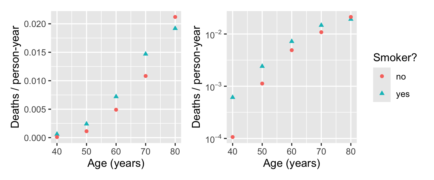
We could choose to model the number of deaths as approximately Poisson, given the death rate: \[ Y \sim \poisson(P f(\beta\T X)), \] so that \(f(\beta\T X)\) represents the rate. If we choose a Poisson GLM with the log link, we could write this as \[ Y \sim \poisson(\exp(\beta\T X + \log P)). \] Here \(P\) is an offset: a term in our model that is fixed to have coefficient 1, rather than having a slope that is estimated. The choice of a Poisson distribution is an approximation here because there is an upper bound to the number of deaths in any age bucket based on the number of people in the study in that age bucket—but as long as the death rate is low, the Poisson distribution will assign very little probability to impossible death numbers.
If this model were true, we’d expect a linear relationship between \(\log(Y/P)\) and \(X\), but the right panel of Figure 13.4 shows this is not linear. We can instead consider a polynomial model. Because the gap between smokers and non-smokers even seems to reverse for the oldest group, we’ll also include an interaction between smoking and age. We use the offset argument to tell R to include the term with coefficient 1.
smoke_fit <- glm(deaths ~ (age + I(age^2)) * smoke,
                 offset = log(py),
                 data = smokers, family = poisson(link = "log"))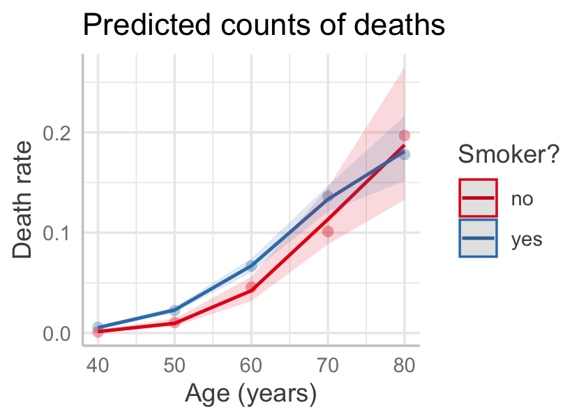
Figure 13.5 gives the effect plot. (Note that predict_response() sets the offset to its mean by default, meaning it used the average of \(\log(P)\); in this case that corresponds to 10,657 person-years.) The fit seems good, though with essentially only ten observations, detailed goodness-of-fit checks may not be useful.
Now suppose we want to compare smokers and non-smokers at age 40, calculating a risk ratio: the ratio of risk of death for smokers versus non-smokers. A simple way would be to make a prediction and take the ratio. To predict the rate of death, we can predict the mean number of deaths for one person-year:
new_smokers <- data.frame(smoke = c("no", "yes"),
                          age = c(40, 40),
                          py = c(1, 1))
preds <- predict(smoke_fit, newdata = new_smokers,
                 type = "response")
preds[2] / preds[1]
2
3.927567 But it’s not easy to make a confidence interval for this. The standard errors are not independent. Let’s more closely examine the regression function—specifically, the ratio between smokers and non-smokers when we set age = 40. The model terms are, in order,
names(coef(smoke_fit))[1] "(Intercept)" "age" "I(age^2)"
[4] "smokeyes" "age:smokeyes" "I(age^2):smokeyes"We can hence write the ratio of predictions as: \[\begin{align*} \frac{\mathbb{E}[Y \mid \text{age} = 40, \text{smoker}]}{\mathbb{E}[Y \mid \text{age} = 40, \text{non-smoker}]} &= \frac{\exp(\hat \beta_0 + 40 \hat \beta_1 + 1600 \hat \beta_2 + \hat \beta_3 + 40 \hat \beta_4 + 1600 \hat \beta_5)} {\exp(\hat \beta_0 + 40 \hat \beta_1 + 1600 \hat \beta_2)} \\ &= \exp(\hat \beta_3 + 40 \hat \beta_4 + 1600 \hat \beta_5) \end{align*}\]
Hence the risk ratio can also be calculated as:
coef_vec = c(0, 0, 0, 1, 40, 1600)

exp(sum(coef_vec * coef(smoke_fit)))
[1] 3.927567We can further create a Wald confidence interval:
se <- sqrt(t(coef_vec) %*% vcov(smoke_fit) %*% coef_vec)[1,1]

bounds <- sum(coef_vec * coef(smoke_fit)) + c(-2, 2) * se
exp(bounds)
[1] 1.49177 10.34059This is quite a large confidence interval, demonstrating the difficulty in estimating risk ratios when the underlying rate of events is so low.
We use an offset because the Poisson distribution is discrete and only supported on the natural numbers; for example, dividing the number of deaths by the number of person-years would result in fractions that are not Poisson, so we could not use that value as a Poisson response variable. We must include the offset in the linear predictor, not account for it in the response.
13.5 Interpretation and inference
Because logistic regression is just a kind of generalized linear model, all the inference techniques we discussed in Section 12.6 apply here. We can conduct Wald tests for coefficients (Theorem 12.3), form confidence intervals for coefficients using the profile likelihood (as in Definition 12.10), and conduct deviance tests to compare nested models (Theorem 12.4).
The key is to keep track of the link function and scales. Let’s consider some common inference tasks.
- Interpreting parameters. In a GLM, the coefficients \(\beta\) relate \(X\) to \(g(\E[Y \mid X = x])\), so interpretation of \(\beta\) depends on the link function \(g\). In logistic regression and binomial GLMs, that is the logit link and we must convert between log-odds and odds ratios (Section 12.3). In a Poisson GLM with the log link, \(\beta\) gives the relationship between \(X\) and the log of the rate, so we must exponentiate it, as we saw in Example 13.6.
- Confidence intervals for parameters. Generally the profile likelihood confidence intervals for \(\beta\) are best; these are produced automatically by
confint(). Again, you can then transform the confidence interval endpoints using the inverse link function. - Making predictions. We can use the
predict()function, but note that thepredict.glmmethod defaults to predicting on the link scale, i.e. predicting \(\hat \beta\T X\). Settype = "response"to have R automatically use the inverse link function to get predictions on the response scale. - Confidence intervals for the mean. If we want a confidence interval for \(\E[Y \mid X = x_0]\), for a particular \(x_0\) of interest, we can get a confidence interval for \(\beta\T x_0\) first. Then we can use the inverse link to transform back. See Example 12.11.
The key, as always, is in interpretation. To interpret a coefficient or a hypothesis test, we need to understand the response distribution and the link function. We must always know if we’re working on the link scale or the response scale, and we must keep track of the appropriate link and inverse link functions for converting back and forth as needed.
Example 13.7 (Deviance test for the smoking data) In Example 13.6, we fit a model for death rate that included a quadratic term for age and an interaction with smoking status. Suppose we wanted a formal hypothesis test to compare a purely additive model (with no quadratic term) to the model we fit. We can use the same techniques introduced for logistic regression in Section 12.6.3.
additive_smoke <- glm(deaths ~ age + smoke, offset = log(py),
                      data = smokers,
                      family = poisson(link = "log"))

anova(additive_smoke, smoke_fit, test = "Chisq")
Analysis of Deviance Table
Model 1: deaths ~ age + smoke
Model 2: deaths ~ (age + I(age^2)) * smoke
Resid. Df Resid. Dev Df Deviance Pr(>Chi)
1 7 69.182
2 4 1.246 3 67.936 1.18e-14 ***
---
Signif. codes: 0 '***' 0.001 '**' 0.01 '*' 0.05 '.' 0.1 ' ' 1We hence reject the null hypothesis that the coefficients for the additional terms (quadratic and interaction) are all zero.
Example 13.8 (Saturated models in GLMs) The deviance of a model was defined in Definition 12.3 by comparing its log-likelihood to the log-likelihood of a saturated model where \(\hat y_i = y_i\) for every observation \(i\). In Example 12.6 we saw that in logistic regression, such a model has log-likelihood 0.
Consider a Poisson regression with log-link instead. When the model is saturated, the predicted rate is always \(\hat y_i = \exp(\hat \beta\T x_i) = y_i\). Substituting in the Poisson mass function, the log-likelihood function for the saturated model is \[\begin{align*} \ell(\beta) &= \sum_{i=1}^n \log f(y_i; x_i, \beta)\\ &= \sum_{i=1}^n \log\left( \frac{y_i^{y_i} \exp(-y_i)}{y_i!} \right)\\ &= \sum_{i=1}^n y_i \log(y_i) - y_i - \log(y_i!). \end{align*}\] This is not zero, and its value depends on the values of \(y_i\) in the data. The log-likelihood attainable by any model, then, depends not just on the quality of the model but the range of \(y_i\), but subtracting out the saturated model’s log-likelihood ensures deviances are more comparable across datasets.
13.6 Overdispersion
It is nice the generalized linear models allow us to model responses as coming from any exponential dispersion family. This allows the variance of \(Y\) to depend on \(X\): in a Poisson GLM, for instance, the variance is proportional to the mean. This can account for the variance patterns in real data.
But sometimes there is overdispersion: there is more variance in \(Y\) than the response distribution would predict. This can happen for several reasons:
- Our \(X\) is not sufficient. The fundamental assumption of a GLM is that each observation \(Y\) is independent and identically distributed given \(X\); but maybe there are other factors associated with \(\E[Y]\) that we did not observe. For a fixed value of \(X\), these other factors may still vary and cause additional variation in the observed values of \(Y\).
- There may be correlation we did not account for. For instance, a \(\binomial(n, p)\) distribution assumes there are \(n\) independent trials—but what if the trials are dependent, and success in one is correlated with increased success rates in the others?
It would be useful if we could fit a more flexible model that allows more variance. We can, by taking advantage of a useful result.
Theorem 13.2 (Mean/variance form of the likelihood equation) For a generalized linear model with canonical link function \(g\) and inverse link \(h = g^{-1}\), the gradient of the log-likelihood can be written as \[ D\ell(\beta) = \sum_{i=1}^n \frac{(y_i - \E[Y_i \mid X_i = x_i]) x_i}{\var(Y_i \mid X_i = x_i)} h'(\beta\T x_i). \] The maximum likelihood estimate is found by setting \(D\ell(\beta) = \zerovec\), so the MLE depends only on the particular exponential dispersion distribution through its mean and variance.
Proof. In Section 13.2, we showed that \[ D\ell(\beta) = \sum_{i=1}^n \frac{(y_i - b'(\beta\T x_i)) x_i}{a(\phi)}, \] while from Theorem 13.1 we know that if \(Y\) has an exponential dispersion family distribution given \(X\), then \[\begin{align*} \E[Y_i \mid X_i = x_i] &= b'(\theta_i)\\ \var(Y_i \mid X_i = x_i) &= b''(\theta_i) a(\phi), \end{align*}\] so \(a(\phi) = \var(Y_i \mid X_i = x_i) / b''(\theta_i)\). If \(g\) is the canonical link (Definition 13.2), then \(\beta\T x_i = \theta_i\). Consequently, we can substitute the mean and variance into the gradient: \[\begin{align*} D\ell(\beta) &= \sum_{i=1}^n \frac{(y_i - \E[Y_i \mid X_i = x_i]) x_i}{a(\phi)}\\ &= \sum_{i=1}^n \frac{(y_i - \E[Y_i \mid X_i = x_i]) x_i}{\var(Y_i \mid X_i = x_i)} b''(\beta\T x_i). \end{align*}\] Finally, note that since for the canonical link \[ b'(\beta\T x_i) = \E[Y_i \mid X_i = x_i] = g^{-1}(\beta\T x_i), \] we’ll need the derivative of the inverse link. For notational convenience, let \(h = g^{-1}\), and then we have \[ b''(\beta\T x_i) = h'(\beta\T x_i). \] This completes the proof.
This result suggests a trick. For any particular GLM with a choice of exponential dispersion distribution, we can write the expectation and variance of \(Y\) in terms of \(X\). Suppose that \[ \var(Y_i \mid X_i = x_i) = v^*(x_i) \] for some function \(v^*\) for the chosen distribution. But suppose that our data is overdispersed. We might instead assume that \[ \var(Y_i \mid X_i = x_i) = \phi v^*(x_i), \] for some constant \(\phi\). If \(\phi > 1\), the data is overdispersed. When we substitute \(\phi v^*(x_i)\) into the likelihood gradient given by Theorem 13.2, we find that \(\phi\) is a constant in every term. Consequently, if the gradient is zero for some value of \(\beta\) when \(\phi = 1\), it will also be zero when \(\phi > 1\). Thus the maximizer \(\hat \beta\) must be the same regardless of \(\phi\).
We can hence use the same MLE for \(\hat \beta\), though this is no longer a model based on a specific distribution function; we are now fudging it and using only the mean and variance of the distribution, and allowing the variance to be different from what an exponential dispersion family distribution would have. Estimation using this approach is hence known as quasi-likelihood estimation, because it only sort of is using a proper likelihood function.
If we further obtain the Hessian of the log-likelihood, as in Section 13.2, we will see that the matrix \(W\) does depend on \(\phi\). From Theorem 12.1, this means \(\var(\hat \beta)\) depends on \(\phi\). Specifically, \(\var(\hat \beta)\) is \(\phi\) times larger than the standard GLM.
Generally we do not know \(\phi\) in advance: we suspect our data is overdispersed, but nature was not kind enough to specify the exact value of \(\phi\) corresponding to the true distribution. We can use a useful property to estimate it.
Theorem 13.3 (Generalized Pearson statistic) Consider data drawn from an exponential dispersion GLM. Then \[ X^2 = \sum_{i=1}^n \frac{(y_i - \E[Y_i \mid X_i = x_i])^2}{\var(Y_i \mid X_i = x_i)} \convd \chi^2_{n - p}. \]
Proof. A heuristic proof: the \(y\)s are conditionally independent, so this is a sum of squared random variables, each centered at 0 and divided by its variance. If each were standard normal, this would be exactly \(\chi^2\); because they are not necessarily normal, the sum is approximately \(\chi^2\).
When using an overdispersed GLM where \(\var(Y_i \mid X_i = x_i) = \phi v^*(x_i)\), we can apply the method of moments to estimate \(\phi\). The expectation of \(X^2\) is \(n - p\), so we set \(X^2 = n - p\) and solve for \(\phi\). We obtain \[ \hat \phi = \frac{1}{n - p} \sum_{i=1}^n \frac{(y_i - \hat{\E}[Y_i \mid X_i = x_i])^2}{\hat v^*(x_i)}. \]
Thus the quasi-likelihood approach is simple: Obtain the MLE \(\hat \beta\) using standard iteratively reweighted least squares, or any other approach; then estimate \(\hat \phi\) as above, and use it to scale the estimated \(\var(\hat \beta)\).
Quasi-likelihood methods are commonly used for Poisson and binomial GLMs when the data is ill-behaved. R supports quasi-likelihood estimation for both by using the quasibinomial() and quasipoisson() families in glm().
Example 13.9 (Overdispersed seeds) Let’s revisit the seed data from Example 13.4 to see how to fit and interpret a quasi-binomial model. In a binomial model, we model \(n_i Y_i\) as binomial, so \(Y_i\) is a proportion. Thus \(n_i y_i\) is the observed number of successes and \(n_i \hat y_i\) is the model’s predicted count, so \(\hat v^*(x_i) = n_i \hat y_i (1 - \hat y_i)\). The overdispersion estimator is \[ \hat \phi = \frac{1}{n - p} \sum_{i=1}^n \frac{(n_i y_i - n_i \hat y_i)^2}{n_i \hat y_i (1 - \hat y_i)}. \] Each term in a sum is a ratio between the observed variance and expected variance for that observation.
We can use quasibinomial() to fit the model:
seed_quasi <- glm(cbind(germinated, total - germinated) ~
                    extract * seed,
                  data = seeds, family = quasibinomial())
We can extract the estimated \(\hat \phi\):
summary(seed_quasi)$dispersion[1] 1.861832And we can also compute it manually from the predicted probabilities \(\hat y_i\):
haty <- predict(seed_quasi, type = "response")
sum((seeds$germinated - seeds$total * haty)^2 /
      (seeds$total * haty * (1 - haty))) / df.residual(seed_quasi)
[1] 1.861832A comparison of this model’s estimates against seed_fit_2 is shown in Table 13.6. Notice that the estimates are identical; only the confidence intervals differ, their width expanding by a constant factor related to \(\hat
\phi\).
| Characteristic |
MLE
|
Quasibinomial
|
||||
|---|---|---|---|---|---|---|
| OR | 95% CI | p-value | OR | 95% CI | p-value | |
| extract | ||||||
| bean | — | — | — | — | ||
| cucumber | 1.72 | 1.05, 2.81 | 0.031 | 1.72 | 0.88, 3.37 | 0.13 |
| seed | ||||||
| aegyptiaca73 | — | — | — | — | ||
| aegyptiaca75 | 0.86 | 0.56, 1.34 | 0.5 | 0.86 | 0.48, 1.58 | 0.6 |
| extract * seed | ||||||
| cucumber * aegyptiaca75 | 2.18 | 1.19, 3.97 | 0.011 | 2.18 | 0.96, 4.94 | 0.080 |
| Abbreviations: CI = Confidence Interval, OR = Odds Ratio | ||||||
Because overdispersed models no longer specify a distribution for \(Y \mid X = x\), various procedures are no longer valid. Tests based on the log-likelihood are not valid because it is not a real log-likelihood; procedures based on simulating new values of \(Y\) (such as lineup plots) cannot be applied; and diagnostics that use the conditional distribution of \(Y\) (such as randomized quantile residuals) do not function.
13.7 Assumptions and diagnostics
When we fit a generalized linear model, we make three key assumptions:
- The observations are conditionally independent, given \(X\).
- The response variable follows the chosen distribution.
- The mean of the response is related to the predictors through the chosen link function and functional form.
We can use residual diagnostics to check the latter two assumptions.
13.7.1 Residuals
As in logistic regression, we can define a variety of residuals for GLMs. The logistic regression residuals introduced in Section 12.5.2 are simply special cases of these, so we can state the general cases without much prelude.
Definition 13.3 (Residuals for GLMs) In a generalized linear model with link function \(g\), the residual for observation \(i\) is \[\begin{align*} \hat e_i &= y_i - \hat{\E}[Y \mid X = x_i] \\ &= y_i - g^{-1}(\hat \beta\T x_i). \end{align*}\]
Definition 13.4 (Standardized residuals for GLMs) In a generalized linear model, the standardized residuals are defined to be \[ r_i = \frac{\hat e_i}{\sqrt{\widehat{\var}(y_i)}}, \] where \(\widehat{\var}(y_i)\) is the estimated variance of the response, given by the selected response distribution. For example, in a Poisson regression, \(\widehat{\var}(y_i) = \hat y_i\), because the variance of a Poisson is equal to its mean.
The standardized residuals are often known as the Pearson residuals.
In logistic regression, we found it difficult to use these residuals in diagnostics because the discrete response variable creates strange patterns in residuals even when the model is well-specified. (See, for instance, Figure 12.7.) Similar problems can affect other GLMs. Depending on the response distribution and the observed range of values, there may only be a few possible values of \(Y\), again creating patterns.
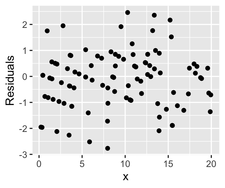
Example 13.10 (Poisson regression residuals) Consider a population in which the true population relationship is \[ Y \mid X = x \sim \poisson(\exp(0.5 + x / 10)). \] This can be fit with a Poisson GLM with log-link. The residuals, shown in Figure 13.6, have a characteristic diagonal banding pattern. Notice that for small values of \(x\), where the mean of \(Y\) is smallest, the bands are farthest apart; for larger values of \(x\), where the mean of \(Y\) is larger and there are hence more possible values, the bands are closer together. When the mean of \(Y\) is large enough, the pattern is impossible to distinguish and the residuals resemble those from linear regression.
While these residuals make reasonable diagnostic plots in some cases, it is easier to use randomized quantile residuals (Section 12.5.4) for all GLMs, rather than switching between residuals depending on the situation. But we can no longer use the simple special case for logistic regression, and must consider the full definition (Definition 12.8). As in logistic regression, the randomized quantile residuals are uniformly distributed when the model is correct.
Let’s consider some examples of randomized quantile residuals in different GLMs with different types of model misspecification.
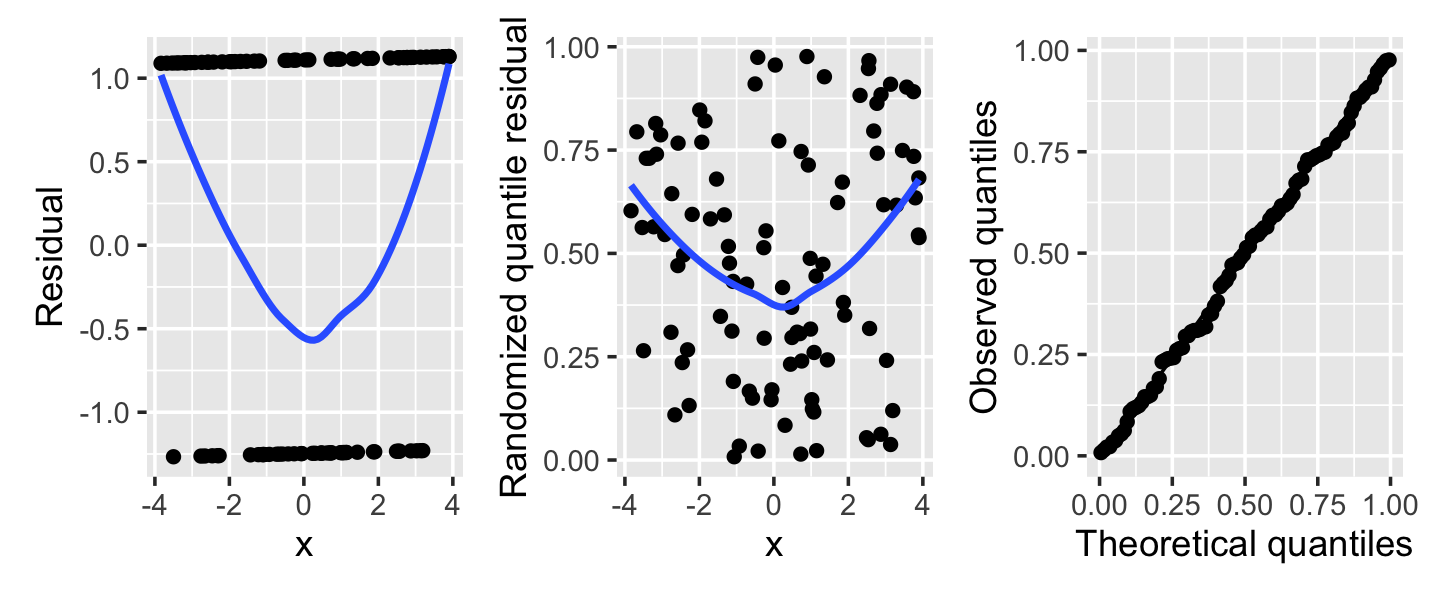
Example 13.11 (Misspecified logistic regression) Consider a logistic regression fit where the true relationship is \[ \log(\odds(Y = 1 \mid X = x)) = \frac{x^2}{4} - 1, \] but we fit a logistic regression assuming a linear relationship. The residuals and randomized quantile residuals are shown in Figure 13.7. The Q-Q plot shows slight deviations from uniformity overall, but more informative is the plot against \(X\), showing a clear U-bend. In the left plot, of ordinary residuals, the trend line is the only informative element—the individual points form two lines that are hard to read. In the center plot, of randomized quantile residuals, the U shape is visible in the residuals directly, making the problem much easier to see.
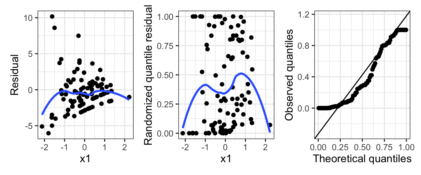
Example 13.12 (Overdispersion in a Poisson regression) Next, consider a population where the true relationship is \[ Y \mid X = x \sim \poisson(\exp(1 - x_1 + x_2)), \] but we fit a Poisson model that does not include \(X_2\). As we saw in Section 13.6, this can create overdispersion: Conditioning on \(X_1\), \(Y\) is a mixture of Poisson distributions with means depending on the particular value of \(X_2\).
The residuals from such a fit are shown in Figure 13.8. Notice in particular that the randomized quantile residuals are not uniformly distributed at all—their values are concentrated towards 0 and 1. This is the tell-tale sign of overdispersion, as it shows that \(Y\) is frequently much larger or much smaller than predicted, and hence has higher variance than the model assumes. A quasi-Poisson fit could fix this, though the ideal solution would be to include \(X_2\) in the model if it is available.
13.7.2 Outliers and influential observations
In Section 9.3.3, we introduced the problems that arise in linear regression when there are outlier observations. There, we understood the problem as a misspecified error distribution: rather than the errors being normally distributed, occasionally one was very large, causing an observation to have an outlying response value.
In a GLM, there is no “error” (in the sense of an error term \(e\) in the model) and no error distribution, but it is still possible to have outliers. An observation may have an usual \(Y\) value that has a large influence on the fitted \(\hat \beta\). In small datasets with a few variables, we can spot such outliers in scatterplots of the data; but in larger datasets they are harder to notice, and so diagnostics are helpful.
One approach would be to adapt the Cook’s distances of linear regression. As we saw in Definition 9.3, the Cook’s distance for an observation measures the change in \(\hat \beta\) resulting from deleting that observation; an observation with a large Cook’s distance hence has large influence on the model fit. We can directly adapt that definition for GLMs.
Definition 13.5 (Cook’s distance for GLMs) In a generalized linear model, the Cook’s distance for an observation \(i\) is defined to be \[ D_i = \frac{(\hat \beta^{(i)} - \hat \beta)\T (\X\T W \X)^{-1} (\hat \beta^{(i)} - \hat \beta)}{p \hat \phi}, \] where \(W\) is the diagonal matrix used in iteratively reweighted least squares (Section 12.2.1) and \(\hat \phi\) is the dispersion parameter (Section 13.6; \(\hat \phi = 1\) when there is no overdispersion).
This has the same interpretation as Cook’s distance in linear models: the change in the estimated parameters, scaled by their variance (which is \((\X\T W\X)^{-1}\) in a GLM; see Theorem 12.1 and following discussion).
In linear models, we did not have to repeatedly refit the model to calculate this—Theorem 9.1 gives a simple formula in terms of the residuals and leverage. Unfortunately, the same is not true for GLMs: the two versions are not equal. Fortunately, Williams (1987) showed that the residuals and leverage can still be used to approximate the change in \(\hat \beta\).
Theorem 13.4 (One-step approximation for Cook’s distances in GLMs) In a generalized linear model, the Cook’s distance for observation \(i\) is approximately \[ D_i \approx r_i^2 \frac{H_{ii}}{p \hat \phi (1 - H_{ii})}, \] where \(H\) is the hat matrix from the last step of IRLS.
Proof. See Williams (1987). The basic idea is to approximate \(\hat \beta^{(i)}\) using a Taylor expansion around \(\hat \beta\); we can then obtain a closed-form approximation for \(\hat \beta^{(i)}\) after one step of IRLS.
This approximation is fairly good, and saves us having to repeatedly re-run IRLS to obtain \(\hat \beta^{(i)}\) for each observation \(i\). It is used by the cooks.distance() function in R when called on GLM fits, and by broom’s augment() to create the .cooksd column.
Exercises
Exercise 13.1 (Gamma distribution) Show that if \(X \sim \operatorname{Gamma}(\alpha, \beta)\), where the gamma distribution has density \[ f(x; \alpha, \beta) = \frac{\beta^\alpha}{\Gamma(\alpha)} x^{\alpha-1} e^{-\beta x}, \] then \(X\) can be written in exponential dispersion form. Provide the functions \(a\), \(b\), and \(c\), and identify the natural parameter.
Exercise 13.2 (Seed germination diagnostics) Figure 13.9 shows the deviance residuals from the interaction model fit in Example 13.4.
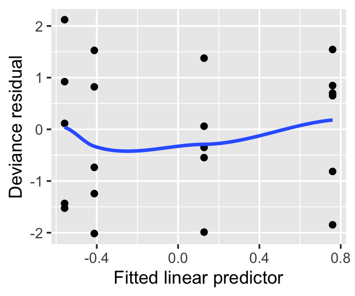
- Why are the residuals grouped in four vertical lines?
- Normally you might use this plot to determine if the modeled mean function is adequate, or if the model needs to include additional terms or flexibility. Explain why that is not necessary or possible here.
Exercise 13.3 (Ant diagnostics) Load the ants data from Example 13.5 and fit the model shown in the example. Use randomized quantile residuals to evaluate the model fit. List the assumptions made by the model, and comment on what the residual plots show about each assumption.
Exercise 13.4 (Island size and extinction rates) The Sleuth3 package contains the data frame case2101, summarizing data originally collected by Väisänen and Järvinen (1977). The data is based on two censuses of nesting birds taken on the Krunnit Islands archipelago in 1949 and 1959. Each row is one island in the archipelago, and we have the number of bird species present in 1949 (AtRisk) and the number of those that were extinct from the island by 1959 (Extinct). As a covariate, we have the area of the island (in hectares2); many of the islands are quite small. Theories of biodiversity would predict that that extinction rates (Extinct / AtRisk) are higher in small, isolated communities, and lower in larger communities.
Conduct an exploratory analysis of the data. Plot extinction rate against area. Also plot the log-odds of extinction rate against both area and the log of area. Comment on the trend in the data.
Describe which GLM you will choose to model extinction rate versus island area (including response distribution and the typical link function). Fill in the blanks: your chosen GLM assumes a linear relationship between the [blank] of the extinction rate and [blank]. Based on that and the plots above, what model and transformation would you use?
Fit your model. In a sentence (in APA format), describe the observed relationship between extinction rate and area. Your sentence should give the odds ratio for extinction associated with an increase in area, and its confidence interval. If you used area on a log scale, describe your odds ratio in terms of area, not log area.
Hint: A one-unit increase in \(\log_{10}(\text{area})\) corresponds to what change in area?
Plot the randomized quantile residuals against your predictor, including a smoothed trend line. Comment on the shape of the residuals. Do you observe any signs of model misspecification?
Exercise 13.5 (Howard the Duck) Howard the Duck is conducting a study to determine whether eating bread is bad for ducks. (The city council wants to know if they should buy “Please Do Not Feed the Ducks” signs.)
Howard enrolls \(n\) ducks in his study and observes them. The outcome variable is how many times each duck was hospitalized during the study period. Covariates include:
- The duck’s age and weight at the start of the study
- How much exercise the duck gets, in miles flown per week
- The fraction of time the duck spends at the public park, where people often throw bread to the ducks.
Howard would like to understand the relationship between being at the public park and the number of hospitalizations for any cause. Howard doesn’t care when the hospitalizations happen, just how many there are.
What type of generalized linear model should be used here? Write out its model for \(Y\) explicitly (e.g., “\(Y\) is Normal with mean given by \(\X\beta\)” in an ordinary linear model).
Suppose that not all ducks are in the study for the same length of time. Some ducks were observed for only a few months, but others were observed for an entire year. Those ducks could obviously be hospitalized more times. How should this be accounted for in Howard’s model? Write out explicitly what you would change in the model.
Howard fit the model and obtained these results:
Coefficients:
              Estimate Std. Error z value Pr(>|z|)
(Intercept) -0.0820563  0.2145272  -0.382    0.702
fraction     0.8714525  0.1645624   5.296 1.19e-07 ***
exercise    -0.0004261  0.0017543  -0.243    0.808
age          0.0865562  0.0167153   5.178 2.24e-07 ***
weight      -0.0491136  0.0474717  -1.035    0.301
---
Signif. codes:  0 ‘***’ 0.001 ‘**’ 0.01 ‘*’ 0.05 ‘.’ 0.1 ‘ ’ 1

(Dispersion parameter taken to be 1)

    Null deviance: 147.936  on 99  degrees of freedom
Residual deviance:  81.468  on 95  degrees of freedom
AIC: 402.62

Number of Fisher Scoring iterations: 4
In a sentence or two, give your conclusions to the city council: do ducks that spend a larger fraction of their time at the public park have worse health? Cite appropriate test statistics and \(p\) values to justify your conclusion in APA format (Chapter 25). Also, state how the rate of hospitalizations changes as the fraction increases by 0.1.
Of course, this was an observational study. Sketch a causal diagram of the variables shown, and suggest a variable not included in the study that could have confounded the results.
Exercise 13.6 (Insect attraction to light) Insects can be attracted to bright artificial lights at night. As cities switched from old-fashioned sodium-vapor street lights (with their characteristic orange glow) to more energy-efficient LED lights, Longcore et al. (2015) wanted to know whether different light sources attract more or fewer insects of different species. They conducted a field experiment using light traps: each trap contained a light bulb and captured insects that were attracted to it.
The experiment used six light traps. Five had different types of light bulb, while one used no light bulb, as a control. The traps were set up each evening at sunset and checked in the morning after sunrise, and the insects in each trap were identified and counted. This process was run 32 times: 16 at an urban site (the UCLA Botanical Garden), 8 times at a rural field station (La Kretz), and 8 times at the rural Stunt Ranch Reserve. The repetitions were done at varying moon phases, since the presence of a bright moon in the sky might affect the results.
The full dataset is available at https://cmustatistics.github.io/data-repository/biology/bug-attraction.html.
We are interested in the total number of insects collected in each trap (the
Totalvariable) and how it relates to the light bulb type (Light Type). We also know that the location (Location), moon phase (% Moon Visible), mean night temperature (Mean Temp), and mean humidity (Mean Humidity) might affect insect activity. Conduct an EDA of these variables to determine what relationships the predictors may have with the response.Consider the study design. Because six traps were placed out each night, each with a different bulb (or no bulb), the traps were exposed to the same location, moon phase, temperature, and humidity. No bulb type has data from moon phases that are systematically different from the other bulbs, or was used on nights that were warmer than those for the other bulbs, or anything like that. This is known as a balanced design.
Comment on what this design choice means. Can location, moon phase, mean temperature, or mean humidity be confounding variables that would bias our estimates of the effect of bulb type? Do we need to incorporate them into our models to obtain an unbiased estimate of the causal effect of bulb type?
Obtain the mean number of insects trapped by each bulb. Display the means in a table. Which bulb attracts the fewest insects?
Note there is one missing count (recorded as
NA) that you may need to remove.Select a GLM for the total number of insects collected as a function of bulb type, location, moon phase, temperature, and humidity. Use your EDA to guide your model choice, and produce any necessary diagnostic plots to validate your choice.
Produce a table of coefficients estimated from your final model, including standard errors. Interpret, in words, the meaning of the coefficient for temperature, giving a 95% confidence interval for the size of the effect.
Consider a night where the moon is 60% visible, the humidity is 60%, and the mean temperature is 15 °C. (These are roughly the average values in the data.) Produce a table of the predicted number of insects trapped by each bulb type at the La Kretz station on a night like this, giving 95% confidence intervals for each prediction. Does your result match the table from part 3?
Exercise 13.7 (Interpreting GLM coefficients) It can be difficult to interpret the coefficients of GLMs with various link functions. Let’s practice different interpretations of various GLMs. In each case below, there is a single predictor \(X\) with coefficient \(\beta_1\), and \(\beta_0\) is the intercept.
Let \(n_i Y_i \mid X_i = x_i \sim \binomial(n_i, g^{-1}(\beta_0 + \beta_1 x_i))\), using the logit link. A 10-unit increase in \(X\) corresponds to what change in the odds of success?
Let \(Y_i \mid X_i = x_i \sim \poisson(g^{-1}(\beta_0 + \beta_1 x_i))\), using the log link. A 2-unit increase in \(X\) corresponds to what change in the mean of \(Y\)?
Let \(Y_i \mid X_i = x_i \sim \poisson(g^{-1}(\beta_0 + \beta_1 \log(x_i)))\), using the log link. (Note the log-transformation of \(x_i\).) Multiplying \(X\) by 10 corresponds to what change in the mean of \(Y\)?
Hint: Recall basic properties of logarithms and exponentials, e.g., \(\log(ab) = \log(a) + \log(b)\). Refer back to Section 7.2 and Section 12.3 for previous examples of how we derived interpretations of coefficients.
Not exactly. The data used here was presented by Crowder (1978), who used it purely to develop a new method for analyzing binomial data, and was not interested in the research question at all. The original research questions posed by Whitney (1978) involved several other species of parasite and types of extract and explored how different concentrations of extract could suppress germination, but that data was not made publicly available, so we’re left with what Crowder (1978) presented.↩︎
Ramsey and Schafer (2013), section 21.1.1, claims the units are square kilometers, but the original source makes clear the area is in hectares. There are 100 hectares in a square kilometer, so this is a large difference.↩︎