8 The Regressinator

The regressinator is an R package that can simulate data from different regression models with different error distributions and population relationships. It can also present different regression diagnostics in “lineup plots”, which help us see how diagnostics can look for well-specified and incorrectly specified models. We will use it throughout the rest of the book for simulations and activities.

library(regressinator)

For more information about the regressinator, including an introductory guide and a reference manual, see its website.

8.1 A good model

To demonstrate how the regressinator works, let’s specify a simple situation where all model assumptions hold. We define a “population”, which specifies the population distribution of $X$, the relationship between $X$ and $Y$, and the distribution of $\epsilon$.

nice_pop <- population(
  x1 = predictor("rnorm", mean = 5, sd = 4),
  x2 = predictor("runif", min = 0, max = 10),
  y = response(
    4 + 2 * x1 - 3 * x2, # relationship between X and Y
    error_scale = 3.0 # errors are multiplied by this scale factor
  )
)

The predictor() function lets us specify the distribution each predictor is drawn from, by naming a function that can be used to draw from it and arguments to provide to that function. The response() function’s first argument is an expression, in terms of the predictors, for the mean of the response, to which errors will be added. (We will define this slightly differently when we get to generalized linear models in Chapter 13.) By default, the errors are drawn from a standard normal distribution, which we can rescale to have different standard deviation using the error_scale argument.

We can use the sample_x() and sample_y() functions to obtain a sample from this population:

nice_sample <- nice_pop |>
  sample_x(n = 100) |>
  sample_y()

head(nice_sample)

Sample of 6 observations from
Population with variables:
x1: rnorm(list(mean = 5, sd = 4))
x2: runif(list(min = 0, max = 10))
y: gaussian(4 + 2 * x1 - 3 * x2, error_scale = 3)

# A tibble: 6 × 3
      x1    x2       y
   <dbl> <dbl>   <dbl>
1  6.74  5.54   -6.88 
2  7.61  8.33  -11.6  
3  3.00  7.87  -12.1  
4  3.15  2.38    5.13 
5  0.948 0.671  -0.591
6 11.8   0.442  25.2

This is an ordinary data frame (just with a couple extra attributes to store population information), and we can easily plot it:

library(ggplot2)

ggplot(nice_sample, aes(x = x1, y = y)) +
  geom_point()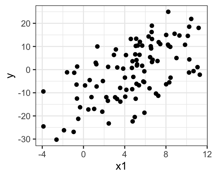

As a demonstration, let’s simulate the sampling distribution of $\hat \beta$. Remember regression inference is usually in the fixed-$X$ setting, so we will use the $X$ values from nice_sample repeatedly; sample_y() will just overwrite the y column. The regressinator provides the sampling_distribution() function to do this automatically. By default, it will repeatedly call sample_y() on the data provided to it, refit the model to that data, and call broom::tidy() to get a data frame of the model coefficients. These data frames are then combined into one large data frame with a .sample column indicating which fit each coefficient came from.

B <- 1000

fit <- lm(y ~ x1 + x2, data = nice_sample)
cis <- confint(fit)

coefs <- sampling_distribution(fit, nice_sample, nsim = B)

Table 8.1: The first few rows of `coefs`, showing estimated coefficients from the original `fit` and the first two simulations.
term	estimate	std.error	statistic	.sample
(Intercept)	3.861	0.695	5.553	0
x1	2.091	0.073	28.797	0
x2	-3.109	0.101	-30.697	0
(Intercept)	3.570	0.722	4.946	1
x1	2.027	0.075	26.897	1
x2	-2.982	0.105	-28.362	1
(Intercept)	4.730	0.795	5.951	2
x1	1.962	0.083	23.638	2
x2	-3.042	0.116	-26.272	2

As we can see in Table 8.1, coefs contains the $\hat \beta$ values from each simulation. There are various ways to extract estimates for specific predictors. For example, using dplyr, we could group by the term column and use summarize() to get means or other summary statistics within each group:

library(dplyr)

coefs |>
  group_by(term) |>
  summarize(mean_se = mean(std.error))

# A tibble: 3 × 2
  term        mean_se
  <chr>         <dbl>
1 (Intercept)  0.696 
2 x1           0.0726
3 x2           0.101

See Wickham and Grolemund (2017) chapter 5 if you are unfamiliar with dplyr and need an introduction. We could alternately use R’s indexing to select a column corresponding to a particular term:

coefs[coefs$term == "x1", "std.error"] |>
  head()

# A tibble: 6 × 1
  std.error
      <dbl>
1    0.0726
2    0.0754
3    0.0830
4    0.0724
5    0.0751
6    0.0600

Data frames are indexed by their rows and columns, so we select the rows by passing a logical vector (coefs$term == "x1") that is TRUE for the rows we want, and we select the column by giving its name.

Exercise 8.1 (Bias and variance) The rows of coefs are, in effect, samples from the population sampling distribution of $\hat \beta$.

Run the code above and analyze coefs to answer the following questions.

Are the estimates biased?
Does the estimate of $\var(\hat \beta)$ provided by vcov(fit) appear reasonably accurate? (You need only check the entries on the diagonal, i.e. the estimated variance of each coefficient, not the covariances.)

Hint: Grouping by the “term” column gives each term in its own group, so you can then use dplyr’s summarize() to get means, standard deviations, and so on.

Exercise 8.2 (Confidence interval coverage) We can get confidence intervals from each model fit as well:

# sampling_distribution uses broom::tidy() to get the
# coefficients, and we can give it `conf.int = TRUE`
# to get CIs
coefs_cis <- sampling_distribution(fit, nice_sample, nsim = B,
                                   conf.int = TRUE)

A 95% confidence interval has correct coverage if 95% of confidence intervals cover (include) the true parameter value. Check if these confidence intervals have approximate 95% coverage.

8.2 Lineups

To help us learn to interpret regression diagnostic plots, the regressinator can produce “lineups”. The lineup process, introduced by Buja et al. (2009), is a way to conduct statistically sound hypothesis tests visually with well-chosen plots, rather than mathematically with well-chosen test statistics. The core idea is simple: If we are looking for a particular pattern in a plot as a sign our null hypothesis is false, then hide the plot among 19 other plots simulated so the null hypothesis is true. If we can distinguish the plot with real data from those where the null hypothesis is true, that is like a test statistic being far from the null distribution; if a test statistic is larger than 19 draws from its null distribution, then $p < 0.05$.

In regression, we can think of the null hypothesis as being that the model is correctly specified. We examine diagnostic plots to determine whether to reject the null (and perhaps make revisions to our model), but it can be difficult to tell if a particular diagnostic plot reveals a real problem or if a pattern we observe is just random noise. Lineups can help us here too (Loy 2021).

The regressinator provides the model_lineup() function. It takes a model fit and does the following:

Get the diagnostics from that model (using augment(), by default)
Simulate 19 additional datasets using the model, using the standard assumptions for that model. (For instance, for linear regression, errors are drawn from a normal distribution.) In each dataset, the same $\X$ values are used, and only new $\Y$ values are drawn. Each dataset is the same size.
For each of those datasets, fit the same model and calculate the diagnostics.
Put the diagnostics for all 20 fits into one data frame with a .sample column indicating which fit each diagnostic came from.
Print out a message indicating how to tell which of the .sample values comes from the original model.

This helps us compare how diagnostic plots will look when assumptions hold (by looking at the 19 simulated datasets) to how the diagnostic plots of our real model look. We can construct a plot using the returned data frame, faceting by the .sample column so we get one plot per simulated (or real) dataset. (If you’re not familiar with ggplot2 and faceting, see chapter 3 of Wickham and Grolemund (2017).)

Exercise 8.3 (Diagnosing a nonlinear trend) Consider a simple dataset where the true relationship is not linear, but we fit a linear model:

nonlinear_pop <- population(
  x1 = predictor("runif", min = 1, max = 8),
  y = response(0.7 + x1**2, family = gaussian(),
               error_scale = 4.0)
)

nonlinear_data <- sample_x(nonlinear_pop, n = 100) |>
  sample_y()

nonlinear_fit <- lm(y ~ x1, data = nonlinear_data)

Since model_lineup() uses augment() on each fit by default, we get fitted values and residuals for each fit. We can plot these and facet by .sample:

model_lineup(nonlinear_fit) |>
  ggplot(aes(x = .fitted, y = .resid)) +
  geom_point() +
  facet_wrap(vars(.sample)) +
  labs(x = "Fitted value", y = "Residual")

decrypt("nsW7 Ykjk l3 gCPljlC3 KR")

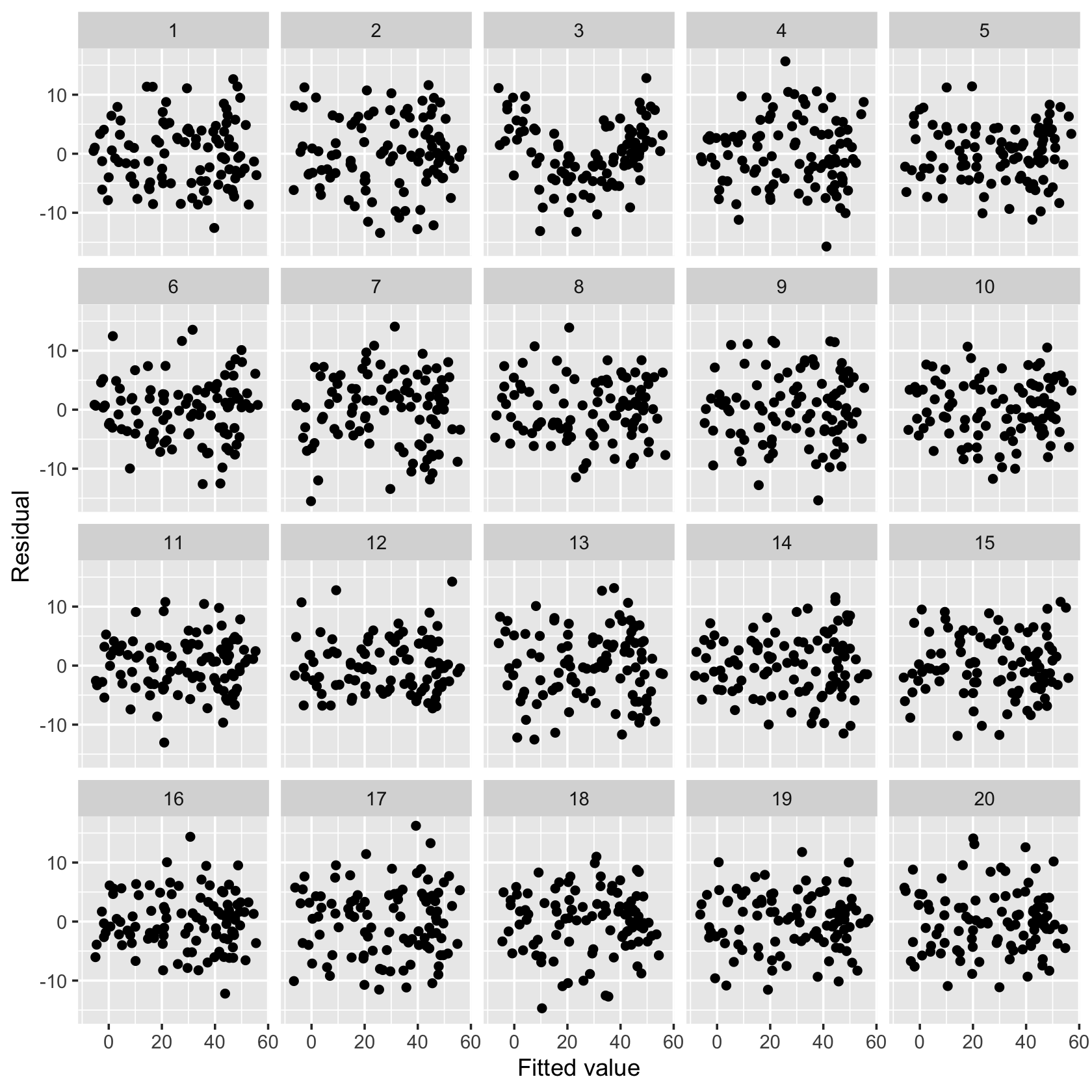
Examine the 20 plots and guess which one represents the model fit to the original data. Paste the decrypt() message into your R console to see if you were right.

We’ll consider more examples of the use of lineup plots to detect model problems in Chapter 9.