characters <- read.csv("data/character-deaths.csv")21 Survival Analysis
\[ \DeclareMathOperator{\E}{\mathbb{E}} \DeclareMathOperator{\R}{\mathbb{R}} \DeclareMathOperator{\RSS}{RSS} \DeclareMathOperator{\AIC}{AIC} \DeclareMathOperator{\bias}{bias} \DeclareMathOperator{\MSE}{MSE} \DeclareMathOperator{\VIF}{VIF} \DeclareMathOperator{\var}{Var} \DeclareMathOperator{\cov}{Cov} \DeclareMathOperator{\cor}{Cor} \DeclareMathOperator{\se}{se} \DeclareMathOperator{\trace}{trace} \DeclareMathOperator{\vspan}{span} \DeclareMathOperator{\proj}{proj} \newcommand{\condset}{\mathcal{Z}} \DeclareMathOperator{\cdo}{do} \newcommand{\ind}{\mathbb{I}} \newcommand{\T}{^\mathsf{T}} \newcommand{\X}{\mathbf{X}} \newcommand{\Y}{\mathbf{Y}} \newcommand{\Z}{\mathbf{Z}} \newcommand{\zerovec}{\mathbf{0}} \newcommand{\onevec}{\mathbf{1}} \newcommand{\trainset}{\mathcal{T}} \DeclareMathOperator*{\argmin}{arg\,min} \DeclareMathOperator*{\argmax}{arg\,max} \DeclareMathOperator{\SD}{SD} \newcommand{\dif}{\mathop{\mathrm{d}\!}} \newcommand{\convd}{\xrightarrow{\mathrm{D}}} \DeclareMathOperator{\logit}{logit} \newcommand{\ilogit}{\logit^{-1}} \DeclareMathOperator{\odds}{odds} \DeclareMathOperator{\dev}{Dev} \DeclareMathOperator{\sign}{sign} \DeclareMathOperator{\normal}{Normal} \DeclareMathOperator{\binomial}{Binomial} \DeclareMathOperator{\bernoulli}{Bernoulli} \DeclareMathOperator{\poisson}{Poisson} \DeclareMathOperator{\multinomial}{Multinomial} \DeclareMathOperator{\uniform}{Uniform} \DeclareMathOperator{\edf}{edf} \]
So far, we have exclusively considered problems of the form “model the relationship between \(X\) and \(Y\)”, where both \(X\) and \(Y\) are completely observed, but we make different assumptions about the distribution of \(Y\) and the shape of the relationship. All of these problems are regression problems, whether our goal is inference or prediction.
Not every problem statistical is of this form, of course. One important class of problems is survival problems: modeling the time until an event occurs, when that time is incompletely observed.
For a detailed reference from a statistician’s point of view, see Aalen et al. (2008).
21.1 Survival setup and censoring
In a survival problem, each unit—each observation—is a person, product, company, or some other thing that can be observed for a length of time. Each unit can experience a certain event a maximum of one time. For example:
- A patient can recover from their illness
- A patient can die from their illness
- A company can go bankrupt
- A product can be returned
- A product can fail
Whatever the event type is in the problem we are studying, in a survival problem we are interested in modeling the rate of that event. We’ll generically call the event “failure” and say that we are interested in modeling failure rates and risks of failure for each unit. (Other sources, such as R’s survival analysis functions, refer to “death” as the generic outcome of interest.)
But this is not simply a binary classification problem, where \(Y \in \{0, 1\}\) and 1 represents failure. We observe each unit \(i\) beginning at time 0, and there are two possible observed outcomes:
- The unit fails at time \(T_i\), known as either the failure time or the survival time (since that is how long the unit survives)
- We reach time \(C_i\) without failure, and no longer observe the unit after that time to know when it fails.
The latter outcome is called censoring, because the true outcome—the true time of failure \(T_i > C_i\)—is censored and unknown to us. Censoring can occur because the study ends, or it can occur because a patient chose to drop out of a study, records became unavailable, or some other problem unrelated to failure; hence different units may have differing censoring times \(C_i\).
TODO diagram like Aalen et al. (2008) fig 1.1
In survival analysis, we are interested in modeling \(T_i\) while accounting for this censoring. Note that survival analysis does not consider outcomes that can occur repeatedly in a unit, although the models for doing so—point processes—are built on many similar concepts.
21.1.1 The basic quantities
The basic quantity of interest is the distribution of \(T\), the survival time. We can define the survival function \[ S(t) = \Pr(T > t), \] which monotonically decreases in time. Because we begin observing every unit at \(t = 0\), \(S(0) = 1\). For some outcomes (like death and taxes), \(S(t)\) declines to 0 as \(t \to \infty\); for other outcomes that do not necessarily happen to every unit, \(S(t)\) declines to some positive value as \(t \to \infty\).
We can also define the hazard rate as \[\begin{align*} h(t) &= \lim_{\Delta t \to 0} \frac{1}{\Delta t} \Pr(t \leq T \leq t + \Delta t \mid T \geq t)\\ &= \lim_{\Delta t \to 0} \frac{1}{\Delta t} \frac{S(t) - S(t + \Delta t)}{S(t)} \\ &= - \frac{S'(t)}{S(t)}, \end{align*}\] which is the instantaneous rate of failure at time \(t\) for units that have survived up to time \(t\). The hazard rate can be any nonnegative function, depending on the outcome of interest.
The cumulative hazard is the integral of the hazard function, \[ \Lambda(t) = \int_0^t h(s) \dif s, \] and will have some useful interpretations later because of its fundamental relationship with the survival function.
Theorem 21.1 (Survival in terms of hazard) For a random variable \(T\) with survival function \(S(t)\) and hazard function \(h(t)\), where \(S(0) = 1\), \[\begin{align*} S(t) &= \exp\left(-\int_0^t h(s) \dif s\right) \\ &= \exp(-\Lambda(t)). \end{align*}\]
Proof. By the chain rule, \[ \frac{d}{dt} \log S(t) = \frac{S'(t)}{S(t)} = - h(t), \] so if we integrate each side from 0 to \(t\), we get \[ \log S(t) - \log S(0) = - \int_0^t h(s) \dif s. \] Because \(S(0) = 1\) and \(\log 1 = 0\), we can exponentiate each side and obtain the desired result.
This relationship implies that if we can estimate the hazard rate, we can produce a matching survival function.
It is helpful to define one more quantity. Let \(Y(t)\) be the set of units at risk immediately before time \(t\); “at risk” means they have not yet failed or been censored.
21.1.2 Common hazards
It can often be useful to think in terms of hazard functions instead of survival functions. Let’s see a few examples to get our bearings.
Example 21.1 (Constant hazard) Suppose that \(h(t) = c\), for some constant \(c > 0\). This implies a constant risk: if you have survived to time \(t_0\), your risk of failure in the next instant is the same as if you had survived to time \(2 t_0\). This property is called “memorylessness”: the failure rate of units currently at risk is independent of their survival time, and the failure process has no memory.
Using Theorem 21.1, we can see that \[ S(t) = \exp\left(-\int_0^t c \dif s\right) = \exp(-c t), \] and so the cumulative distribution function is \(F(t) = 1 - S(t) = 1 - \exp(-ct)\). This is the cumulative distribution function of an exponentially distributed random variable. In other words, if the failure time is exponentially distributed, the hazard rate is constant.
TODO increasing, decreasing, constant, bathtub hazards; example plots of hazards and survivals together
21.1.3 The problem of censoring
If we completely observed failure times for all units—if no units were censored—we could trivially estimate \(S(t)\) by the same technique as we use to estimate an empirical cumulative distribution function (Definition 15.1). That is, our estimator could be \[ \hat S(t) = 1 - \hat F(t) = \frac{1}{n} \sum_{i=1}^n \ind(T_i \geq t). \]
But the presence of censoring makes the problem much more challenging. Our estimators of survival and hazard functions are dependent on \(Y(t)\), the risk set at time \(t\), and will compare the number of events in an interval to the risk set to estimate failure rate. (That is, after all, all they can do without making parametric assumptions about the distributions of survival and censoring times, because the risk set and observed failures are all we have.)
For inferences based on observed failures and the risk set to be generalizable, however, we must have independent censoring.
Definition 21.1 (Independent censoring) In a survival problem, censoring is independent if, at any time \(t\), the hazard \(h(t)\) for units in the risk set \(Y(t)\) is identical to the (unobserved) hazard \(h_C(t)\) for the completely observed survival process, i.e. the process with no censoring.
Independent censoring implies that those at risk at time \(t\) are representative of all units: their survival time distribution is no different than the units that were censored before time \(t\).
Independent censoring is a key assumption that is used by all the survival methods we will discuss.
21.2 Nonparametric survival estimators
Despite the failure of the empirical survival function in the presence of censoring, we can still construct a nonparametric estimator of the survival function. The most common is the Kaplan–Meier estimator.
Consider the survival function at time \(t\). Divide up the time interval \([0, t)\) into \(K\) small bins, say \([0, \tau_1), [\tau_1, \tau_2), \dots, [\tau_{K-1}, \tau_K)\), where \(\tau_K = t\). Then by the properties of conditional probabilities, \[ S(t) = \prod_{k=1}^K S(\tau_k \mid T > \tau_{k - 1}). \] Each term in the product is the probability of survival to time \(\tau_k\) for units that survive past \(\tau_{k-1}\). If we choose the intervals to be small enough that each contains only one event—say, if we let \(\tau_1 < \tau_2 < \dots < \tau_K\) be the ordered times of observed events—then it is easy to estimate each term, because we know the risk set in the interval and we know the number of events (one). This leads to the Kaplan–Meier estimator.
Definition 21.2 (Kaplain–Meier estimator) Given \(n\) units, of which \(K\) failed without censoring, the Kaplan–Meier estimator of the survival function is \[ \hat S(t) = \prod_{T_j \leq t} \left( 1 - \frac{1}{|Y(T_j)|} \right). \]
The Kaplan–Meier estimator is sometimes known as the product-limit estimator.
TODO plot some examples in R
TODO asymptotic distributions?
A different approach is to consider estimating the cumulative hazard function \(\Lambda(t)\), and from this estimate calculate the survival curve or the hazard. Again, suppose there were \(n\) units, \(K\) failures, and ordered failure times \(\tau_1 < \tau_2 < \dots < \tau_K\). Consider a small time increment \([t, t + \Delta t)\), with \(\Delta t\) chosen so the interval contains at most one event. By definition of the hazard rate, the probability of an event in this time interval among units that have not already failed is \(h(t) \Delta t\). We can estimate this by dividing the number of failures in the interval by the number of units at risk.
The cumulative hazard is the integral of the hazard; thinking of it as a Riemann sum, it is the sum of \(h(t) \Delta t\) for many such small intervals. For intervals containing no events, our estimate of the hazard in that interval is zero, so those intervals do not contribute to the sum. Instead we can sum up just the intervals containing observed events. This leads to a simple estimator.
Definition 21.3 (Nelson–Aalen estimator) The Nelson–Aalen estimator of the cumulative hazard \(\Lambda(t)\) is \[ \hat \Lambda(t) = \sum_{T_i \leq t} \frac{1}{|Y(T_i)|}. \]
To obtain an estimated survival function, we can apply Theorem 21.1; to obtain an estimated hazard function, we could apply a nonparametric smoother to this curve and take its derivative. (Smoothers based on polynomials, for example, are easy to calculate exact derivatives for.)
21.3 Hazard models
Of course, in many settings we are interested in how each unit’s covariates are associated with its survival. While nonparametric survival estimators are useful, they do not directly help us answer this question—except perhaps if the covariate of interest is categorical, and we can separately estimate and plot the survival functions for each group.
We could of course create parametric models for \(S(t)\) and relate the parameters to covariates for each unit, then fit the model via maximum likelihood. If the model for \(S(t)\) has parameter vector \(\beta\), we could write a likelihood function: \[ L(\beta) = \left(\prod_{i \text{ uncensored}} f(T_i)\right) \left(\prod_{i \text{ censored}} S(C_i)\right), \] where \(f\) is the density function of the parametric survival time distribution. But this requires an exact parametric form for the distribution, which is quite limiting.
As we will see, however, we can define and fit models for the hazard function \(h(t)\), and can easily fit what are called “semiparametric” models, meaning the exact functional form of \(h(t)\) need not be specified. The most common class of models are what are called relative risk regression models, because they model \[ h(t \mid X_i = x_i(t)) = h_0(t) r(x_i(t)). \] Here \(h_0(t)\) is a baseline hazard function, and the hazard for any particular unit is multiplied by \(r(x_i(t))\). Note that here the covariates may change over time. If we can estimate \(r\), we can obtain hazard ratios: the ratio of hazards between two units with different covariate values. This is sometimes called the relative risk, though strictly speaking risks are the cumulative probability of an outcome, not the instantaneous hazard.
There are many possible choices of \(h_0(t)\) and \(r(x_i(t))\). Let’s consider some common models.
21.3.1 Cox proportional hazards model
For simplicity, suppose the covariates are fixed in time; and to ensure that \(h(t) > 0\), let \[ r(x_i) = \exp(\beta\T x_i). \] This is the Cox proportional hazards model (Cox 1972). It assumes that covariates influence the hazard through a specific link function (the exponential). If we can estimate \(\beta\), we can calculate hazard ratios and describe how covariates are associated with hazard. How do we estimate it?
Again, if we wrote down a parametric form of \(h_0(t)\), we could use maximum likelihood. But Cox’s clever trick was to realize that we do not need to write down \(h_0(t)\). (TODO rate, not probability?) Instead, consider the conditional probability \(\Pr(T_i = t \mid Y(t), \text{one failure at } t)\), the probability that unit \(i\) fails at \(t\) given that one unit fails at \(t\) and given the set at risk at \(t\). We can write this as \[\begin{align*} \Pr(T_i = t \mid Y(t), \text{one failure at } t) &= \frac{\Pr(T_i = t \mid Y(t))}{\Pr(\text{one failure at } t \mid Y(t))}\\ &= \frac{h(t \mid X_i = x_i)}{\sum_{j \in Y(t)} h(t \mid X_j = x_j)} \\ &= \frac{\exp(\beta\T x_i)}{\sum_{j \in Y(t)} \exp(\beta\T x_j)}. \end{align*}\] Notice that the baseline hazard \(h_0(t)\) cancels out of this expression.
Now we need to obtain a likelihood for \(\beta\). Again, if we observed \(K\) failures out of \(n\) units, and the failure times are ordered as \(\tau_1 < \tau_2 < \dots < \tau_K\), the product of these conditional probabilities is \[ L(\beta) = \prod_{i=1}^K \frac{\exp(\beta\T x_i)}{\sum_{j \in Y(\tau_i)} \exp(\beta\T x_j)}. \] This is referred to as the partial likelihood for \(\beta\). It is called the partial likelihood because multiplying the probabilities does not give us the unconditional probability density we would usually use in a likelihood; it is conditional on the total number of failures and their times. In other words, given the number of failures and their times, we are measuring the probabilities of particular orderings for the failing units, based on their covariates.
Nonetheless, the maximum partial likelihood estimator \[ \hat \beta = \argmax_\beta L(\beta) \] behaves much like any other maximum likelihood estimator: it is unbiased, consistent, and asymptotically normally distributed (Tsiatis 1981).
Interpretation of coefficients in the Cox proportional hazards model is relatively straightforward: a one-unit increase in \(X_j\) is associated with a hazard that is a factor of \(\exp(\beta_j)\) times larger, meaning the failure rate is \(\exp(\beta_j)\) times higher. This is known as a hazard ratio, and is generally easier to interpret than, say, an odds ratio, even though it is not a probability.
Example 21.2 (Survival in A Song of Ice and Fire) A Song of Ice and Fire is a series of fantasy novels by George R.R. Martin, well-known for their television adaptation as Game of Thrones. They are also well-known for their brutality: many characters are introduced, become important, and then are suddenly killed.
The data file character-deaths.csv contains each character introduced in the book series and the chapter of their death, measured from the beginning of the series. (This data was collected by Erin Pierce and Ben Kahle.) We are interested in the survival function from the perspective of a reader: what is the death rate for characters, measured per chapter, rather than in the internal timeline of the novels? Each character in the file has some additional data indicating their gender, their nobility, their house of allegiance, and various other useful information for readers of the books.
There are 917 characters in the data file. To fit a survival model in R, we load the survival package (included with R). We must tell it each character’s death or censoring time, and whether the character died or was censored; here, the Time column either gives the chapter of death or the last chapter of the book series, and Death indicates whether the character died or was censored.
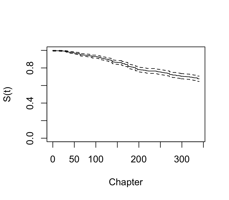
First, let’s use survfit() to fit a Kaplan–Meier survival curve for all characters. We use Surv() to represent the failure and censoring information.
library(survival)

survive <- survfit(Surv(time = Time, event = Dead) ~ 1,
                   data = characters)
There is a plot() method for survfit() objects, and the result is shown in Figure 21.1. We see that over 20% of characters died by the end of the series, and there are numerous jumps indicating deaths of multiple characters.
We can also consider stratifying by gender and nobility. If we give a formula, the curves will be fit for each combination of gender and nobility status:
strat_survive <- survfit(Surv(time = Time, event = Dead) ~
                           Gender + Nobility,
                         data = characters)
strat_survive
Call: survfit(formula = Surv(time = Time, event = Dead) ~ Gender +
Nobility, data = characters)
2 observations deleted due to missingness
n events median 0.95LCL 0.95UCL
Gender=Female, Nobility=Commoner 73 24 NA NA NA
Gender=Female, Nobility=Noble 84 9 NA NA NA
Gender=Male, Nobility=Commoner 412 164 NA NA NA
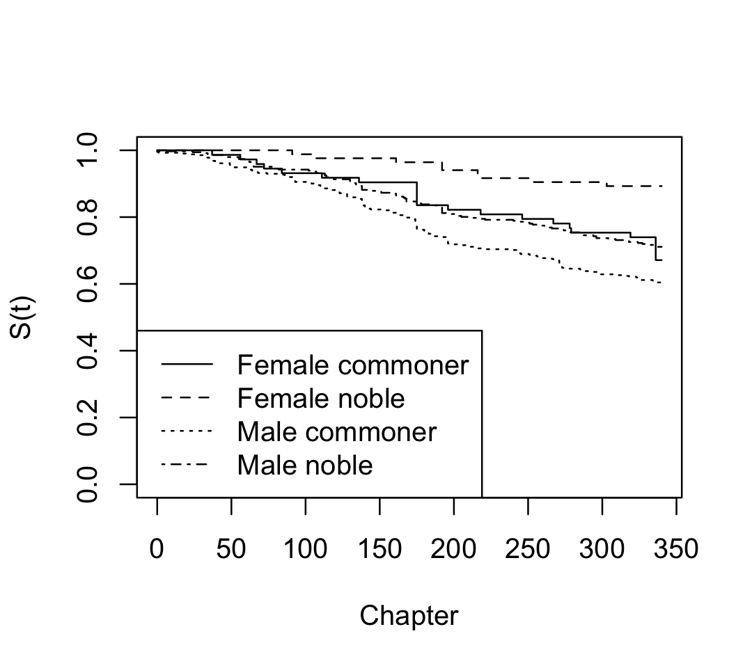
Gender=Male, Nobility=Noble 346 100 NA NA NAWe can see that the books are male-dominated; but from the survival curves plotted in Figure 21.2, we can also see that male characters have much worse survival rates. Notice that plot() does not include confidence intervals automatically when plotting multiple survival curves at the same time, as it would become confusing.
Now let’s fit a Cox proportional hazards model so we can quantify the differences as hazard ratios. Here we are not including an interaction term:
fit <- coxph(Surv(time = Time, event = Dead) ~
               Gender + Nobility,
             data = characters)
The hazard ratios (exponentiated coefficients) are shown in Table 21.1. We see that male characters have higher risks of death, while noble characters have lower risks; both effects are statistically significant, meaning the confidence interval does not include a hazard ratio of 1. Notice there is no intercept, because the intercept is absorbed into the baseline hazard \(h_0(t)\), which we have not estimated.
| Characteristic | HR | 95% CI | p-value |
|---|---|---|---|
| Gender | |||
| Female | — | — | |
| Male | 1.79 | 1.24, 2.57 | 0.002 |
| Nobility | |||
| Commoner | — | — | |
| Noble | 0.61 | 0.48, 0.78 | <0.001 |
| Abbreviations: CI = Confidence Interval, HR = Hazard Ratio | |||
Once we’ve fit a Cox proportional hazards model, we can interpret the coefficients \(\hat \beta\) as desired, but we may also want to estimate the baseline hazard \(h_0(t)\) or the survival curve \(S(t \mid X = x)\) for specific covariate values. The baseline hazard was, of course, deliberately not estimated by the partial likelihood maximization, so we will need to estimate it. The most common method is to estimate the cumulative baseline hazard function.
Definition 21.4 (Breslow estimator) We can estimate the cumulative baseline hazard function \(\Lambda_0(t) = \int_0^t \lambda_0(s) \dif s\) by the quantity \[ \hat \Lambda_0(t) = \sum_{T_i \leq t} \frac{1}{\sum_{j \in Y(T_i)} r(x_j(T_i))}. \] This nonparametric estimate can be motivated by a similar argument as the Nelson–Aalen estimator of the cumulative hazard (Definition 21.3).
Consequently, the cumulative hazard for an individual with particular covariates \(x_0\) can be estimated by \[ \hat \Lambda(t \mid X = x_0) = \hat r(x_0) \hat \Lambda_0(t), \] where \(\hat r(x_0)\) is the estimate from the Cox model.
Through Theorem 21.1, we can also use this to estimate the survival function for an individual with particular covariate values.
21.4 Interpretation
In the Cox proportional hazard model, we can calculate hazard ratios for any desired change in covariates, such as increasing a covariate by one: \[ \frac{h(t \mid X_1 = \textcolor{red}{x_1 + 1}, \dots, X_p = x_p)}{h(t \mid X_1 = \textcolor{red}{x_1}, \dots, X_p = x_p)} = \frac{h_0(t) \exp(\beta_0 + \beta_1 (x_1 + 1) + \dots + \beta_p x_p)}{h_0(t) \exp(\beta_0 + \beta_1 x_1 + \dots + \beta_p x_p)} = \exp(\beta_1). \] Regression coefficients are usually presented already exponentiated, as the original form is difficult to interpret. Hazard rates are deceptively simple. They are easy to quote in text, as is in this recent study:
In the multiple Cox proportional hazard model, patients admitted during the weekend had a significantly higher cumulative risk of death compared to those admitted on the weekdays (AHR, 1.28, 95% CI, 1.21, 1.75, P value = 0.01). (Arega et al. 2024)
Here AHR means “adjusted hazard ratio”, referring to hazard ratios from the Cox model controlling for confounders. But we can’t directly say that the risk of death is 1.28 times higher for patients admitted on weekends; after all, the risk of death is 1, given enough observation time. We also can’t directly interpret this as giving a ratio of times, such as saying patients admitted on weekends die 1.28 times sooner. The direct interpretation is that at any instant after admission, a patient who is still alive has 1.28 times higher risk of death if they were admitted on a weekend. Converting this to any other quantity would require integrating over time—which would require \(h_0(t)\).
There is one available interpretation as the probabilistic index.
Theorem 21.2 (Probabilistic index) If we have units \(i\) and \(j\) with covariate vectors \(X_i, X_j\) and failure times \(T_i\), \(T_j\), then \[\begin{align*} \odds(T_i < T_j \mid X_i, X_j) &= \exp(\beta\T (X_j - X_i)) \\ \Pr(T_i < T_j \mid X_i, X_j) &= \frac{1}{1 + \exp(\beta\T(X_j - X_i))}. \end{align*}\] The hazard ratio is hence the odds for the event \(T_i < T_j\).
Proof. De Neve and Gerds (2020), appendix A.
In the hospital admission data, for example, the probability a patient admitted on the weekend dies sooner than a patient admitted on a weekday (holding other covariates fixed) is \(1 / (1 + \exp(-1.28)) = 0.78\).
As relative risks, it is also important to interpret the Cox model coefficients while keeping in mind that the baseline risks also vary between groups.
Example 21.3 (Hazard ratios of smoking) Since the 1960s, there have been numerous studies on the health effects of tobacco smoking. (We examined one such study in Example 13.6.) Cigarettes first became popular after World War I, and in the 1920s through 1940s expanded dramatically in popularity. But this popularity was, at least at first, primarily among men: smoking was seen as improper, immoral, or impolite for women. Smoking rates among women caught up to men only later, in the 1960s and onwards, as social norms changed and cigarette manufacturers began deliberately advertising cigarettes to women as liberating them from constrictive social norms (Brandt 2007).
This meant that studies comparing the effects of tobacco by gender came much later, once women were smoking at rates similar to men. One such study used cohorts recruited in the 1970s and 1980s, tracking them for years to see which cohort members had heart attacks (Prescott et al. 1998). The study fit a Cox proportional hazards regression model and reported the following results:
Female current smokers had a relative risk of 2.24 (range 1.85–2.71) and male smokers 1.43 (1.26–1.62) relative to non-smokers. This difference was significant (ratio 1.57 (1.25–1.97), P=<0.001) and was not changed after multiple adjustment for other risk factors.
Because the relative risks were higher for women, the authors concluded “Women may be more sensitive than men to some of the harmful effects of smoking.”
But Perneger (1998), in a letter to the editor, pointed out that this conclusion does not follow. In the study, the relevant sample sizes were:
| Smokers | Non-smokers | |
|---|---|---|
| Men | 8490 | 4701 |
| Women | 6461 | 5011 |
Of the women, 512 had heart attacks during the study; of the men, 1,251 did. Because there was little censoring, Perneger could work out the base rate of heart attack in each group from these sample sizes, and reach the following conclusions:
…We can calculate that in women the risk of developing myocardial infarction [heart attack] during follow up is 5.88% (380/6461) in smokers and 2.63% (132/5011) in non-smokers; in men, the risk is 10.62% (902/8490) in smokers and 7.38% (349/4701) in non-smokers… The difference that is attributable to smoking was therefore 3.25% in women and 3.24% in men. Over 12 years, smoking caused an additional myocardial infarction in one person out of 31—equally distributed between men and women.
In other words, because the baseline risks were different, a nearly identical change in absolute risk corresponded to a relative risk that was different between men and women. This demonstrates that we must be very careful when interpreting coefficients in multiplicative models, like the Cox proportional hazards model (and like logistic regression and Poisson GLMs), since the size of a multiplicative change depends on the baseline size as well.
And while another letter misinterpreted the finding still further to say that “women who smoke are at 50% greater risk of myocardial infarction than men who smoke” (Woll 1998), the risk for men was higher than for women, in both smokers and non-smokers. A higher relative risk is not a higher absolute risk.
Similarly, in another letter about the same paper, Tang and Dickinson (1998) pointed out that:
The relative risk due to smoking, for example, is much higher for lung cancer than heart disease—lung cancer has few other causes, but smoking kills more people through heart disease because this disease is much more common, so the additional absolute risk (the attributable risk) of heart disease is much greater.
If you smoke, your risk of lung cancer is a very small number (the baseline hazard) times a large number (the relative risk for smoking); your risk of heart disease, however, is a moderately large number (the baseline hazard) times a moderately large number (the relative risk for smoking). Smoking can hence cause more cases of heart disease each year than cases of lung cancer, despite the relative risk being higher for lung cancer.
21.5 Diagnostics
The Cox proportional hazards model makes several assumptions (that hazards are proportional and the proportionality is associated with specific covariates in a specific way; independent censoring is also required, but untestable) that we would like to be able to check.
We would like some definition of residuals that we can plot here, but it is not obvious what kind of residual to define. We are not making point predictions of failure times for each unit that we could compare to the observed failure times; we are estimating a distribution, or a hazard rate.
Instead, the cumulative hazard function \(\Lambda(t)\) can be used to calculate residuals in common survival models (Therneau et al. 1990).
Definition 21.5 (Martingale residuals) For a survival process with observed censoring times \(C_i\) and failure times \(T_i\), the martingale residuals are defined to be \[ M_i = \ind(i \text{ failed}) - \Lambda(\min\{C_i, T_i\} \mid X_i = x_i). \] These residuals can be estimated by calculating \(\hat \Lambda(t) = \int_0^t \hat h(s) \dif s\).
An intuitive interpretation is that these residuals compare the number of observed events for each unit \(i\) against the expected number under the model, given by \(\hat \Lambda\); it is not exactly correct to think of \(\hat \Lambda\) as an expected number of events, but it is close enough for our purposes.
These residuals have useful properties: when the model is well-specified, they sum to zero, have mean zero, and have no covariance (at least asymptotically). The derivation of these properties requires the theory of martingales; see Therneau et al. (1990) or Aalen et al. (2008), section 4.1.3.
On the other hand, these residuals suffer from similar problems as in logistic regression: because the outcome either occurs or does not occur, the distribution of martingale residuals can be quite skewed and clumped. This behavior also depends on the number of censored observations. As in logistic regression, it can be more useful to smooth or bin the residuals, such as by plot the residuals against a covariate with a smoothing line superimposed.
For overall measures of model performance, we don’t have an equivalent of overall squared error or accuracy—we are predicting the rate of events, not their number or whether they occur. But the probabilistic index above (Theorem 21.2) suggests a way of scoring the predictions from a Cox proportional hazard model, called the concordance index (Harrell et al. 1982).
Definition 21.6 (Concordance index) Enumerate every pair of units in the data where at least one unit had a failure. The concordance index \(c\) is the fraction of all such pairs where the unit with the earlier failure had a higher hazard.
If \(c = 0.5\), the survival model is essentially guessing which unit is likely to fail first; if \(c = 1\), the covariates are sufficient to always determine which unit will fail first. This can be used as a measure of goodness-of-fit or predictive performance. It can also be used for methods beyond survival analysis: for any analysis that provides some kind of risk score for each unit (such as a logistic regression predicting probability of failure), we can use the concordance index to determine if the risk score is indeed higher for units that fail earlier.
21.6 Using classifiers
Exercises
Exercise 21.1 (Inadvertent perioperative hypothermia) Review the dataset description at https://cmustatistics.github.io/data-repository/medicine/core-temperature.html.
Answers the questions under the “Survival analysis” heading to conduct a survival analysis for time spent in the hospital. Give your interpretation in the form of a short Results section of a report: give the table of coefficients and a paragraph of interpretation, explaining whether inadvertent perioperative hypothermia is associated with longer duration in the hospital.