22 Missing Data
\[ \DeclareMathOperator{\E}{\mathbb{E}} \DeclareMathOperator{\R}{\mathbb{R}} \DeclareMathOperator{\RSS}{RSS} \DeclareMathOperator{\AIC}{AIC} \DeclareMathOperator{\bias}{bias} \DeclareMathOperator{\MSE}{MSE} \DeclareMathOperator{\VIF}{VIF} \DeclareMathOperator{\var}{Var} \DeclareMathOperator{\cov}{Cov} \DeclareMathOperator{\cor}{Cor} \DeclareMathOperator{\se}{se} \DeclareMathOperator{\trace}{trace} \DeclareMathOperator{\vspan}{span} \DeclareMathOperator{\proj}{proj} \newcommand{\condset}{\mathcal{Z}} \DeclareMathOperator{\cdo}{do} \newcommand{\ind}{\mathbb{I}} \newcommand{\T}{^\mathsf{T}} \newcommand{\X}{\mathbf{X}} \newcommand{\Y}{\mathbf{Y}} \newcommand{\Z}{\mathbf{Z}} \newcommand{\zerovec}{\mathbf{0}} \newcommand{\onevec}{\mathbf{1}} \newcommand{\trainset}{\mathcal{T}} \DeclareMathOperator*{\argmin}{arg\,min} \DeclareMathOperator*{\argmax}{arg\,max} \DeclareMathOperator{\SD}{SD} \newcommand{\dif}{\mathop{\mathrm{d}\!}} \newcommand{\convd}{\xrightarrow{\mathrm{D}}} \DeclareMathOperator{\logit}{logit} \newcommand{\ilogit}{\logit^{-1}} \DeclareMathOperator{\odds}{odds} \DeclareMathOperator{\dev}{Dev} \DeclareMathOperator{\sign}{sign} \DeclareMathOperator{\normal}{Normal} \DeclareMathOperator{\binomial}{Binomial} \DeclareMathOperator{\bernoulli}{Bernoulli} \DeclareMathOperator{\poisson}{Poisson} \DeclareMathOperator{\multinomial}{Multinomial} \DeclareMathOperator{\uniform}{Uniform} \DeclareMathOperator{\edf}{edf} \]
Gelman et al. (2021), sections 17.3-17.6, or ARM chapter 25 http://www.stat.columbia.edu/~gelman/arm/missing.pdf
Missingness is a common problem in data analysis. Often, one observation will have some but not all of its variables known, for various reasons:
- Respondents don’t always respond to every question on a survey, but instead skip some or stop taking the survey before they’re finished
- Doctors don’t order every test for every patient, so some test results are only available for some patients
- Sometimes samples are lost or the measurement instrument fails
- Some data comes from news reports, public records, and other data sources that are often incomplete.
This kind of missingness is different from sampling bias, where some units are never observed because they were not in our sample, perhaps in a systematically biased way. In missingness, we observe some attributes of the units, but not all of them.
If we ignore missingness—such as by simply throwing away incomplete observations—we can often bias our analyses and draw the wrong conclusions. More careful approaches are needed, although as we will see, missingness is often an intractable problem: we cannot test the accuracy of a method for dealing with missing data, because by definition, we do not know the truth.
There are different types of missingness, and their implications are different, so let’s consider them first.
22.1 Types of missingness
As a motivating example, let’s consider a project I helped run: the US COVID-19 Trends and Impact Survey (Salomon et al. 2021). During the COVID pandemic, from April 2020 to June 2022, Facebook invited a random sample of its users to take this survey, which we hosted and ran at CMU. (For the moment, let’s ignore the possible bias introduced by some respondents refusing to take the survey; we will return to this in Section 22.3.) The survey asked respondents various questions about any symptoms they were experiencing, their mental health, whether they were participating in in-person activities, their attitudes toward vaccination, and various other topics; this data has been used for COVID forecasting work and numerous research projects on the impacts of COVID.
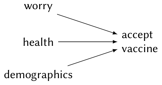
One research question of particular interest in early 2021, when COVID vaccines first became available, was how different factors predict an individual’s willingness to get vaccinated. Public health officials expected that demographics (such as age, gender, and race) would affect vaccine acceptance, but also that other individual features might: whether a person had serious health conditions, whether they were worried about COVID affecting them and their family, and so on. One plausible causal diagram is shown in Figure 22.1.
But respondents don’t all answer every question on the survey. In early 2021, the vaccination questions were early in the survey, but the demographic questions came later. None of the questions were mandatory, so it was possible to skip questions without providing an answer; and since respondents were participating voluntarily, about 20% of them stopped taking the survey before reaching the end. This caused substantial missingness. In surveys, this kind of missingness is also known as item non-response.
Following a framework introduced by Daniel et al. (2012), we can model missingness as part of our causal diagram by adding nodes representing whether variables are missing. For example, we can add a node \(R\) to indicate if all variables of interest were observed. Let \(R = 1\) if all variables are observed and \(R = 0\) if any are not observed. When we complete our analysis by throwing away observations with missing data, we are implicitly conditioning on \(R = 1\).
For example, suppose the servers hosting the online survey occasionally crashed, causing people to be unable to complete the survey after they had started and answered several questions. Suppose this occurred at random times of day, and was not caused by any specific responses by any specific respondents. We can represent this by adding \(R\) to the causal diagram. In this case, because \(R\) is not caused by any other nodes, it is not connected to them. The missing variables are hence missing completely at random.
Definition 22.1 (Missing completely at random) A variable \(X\) is missing completely at random (MCAR) if its missingness is independent of all other observed variables. That is, if \(R\) is an indicator of whether \(X\) is missing, \(R\) is independent of all observed variables. In a causal diagram, \(R\) is disconnected from the graph.
We can see intuitively from the diagram that conditioning on \(R=1\) will not induce any spurious associations between variables in the graph. In other words, we can do a complete cases analysis: analyze only the observations where the relevant variables were fully observed. Because the missingness is independent of all the variables, this is the same as taking a random sample of our sample, and so our analysis would be unbiased for the same reason that an analysis of a random sample is a valid way to make estimates for the population.
In R, most modeling functions (such as lm() and glm()) automatically do a complete cases analysis when given data with missing values (NAs); see the documentation for their na.action argument. There is usually no warning that this is happening, so it is important to check the data for missingness before your analysis so you understand what R is doing.
Suppose instead that in early 2021, when young people were not yet eligible to receive COVID vaccines, they were more likely to skip the vaccination questions because they felt irrelevant—but continued to complete other questions, such as the demographic questions. We can again represent this in a causal diagram, but there is now an arrow to \(R\), as shown in Figure 22.2.
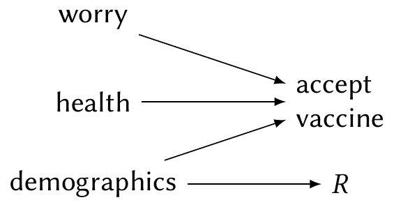
In this case, the missingness is not “completely” random: the probability of missingness depends on a variable in our data. Crucially, that variable is one we observe, so even when the vaccine question responses are missing, we know the respondent’s age. In this case, the vaccination variables are missing at random.
Definition 22.2 (Missing at random) A variable \(X\) is missing at random (MAR) is its probability of missingness depends only upon observed variables that are not missing. That is, if \(R\) is an indicator of whether \(X\) is missing, \(R\) is connected only to nodes in the causal graph that are observed.
Do not confuse MCAR with MAR, despite their similar names.
As we can see informally from the diagram, conditioning on demographics blocks the path between \(R\) and any other variable; it would seem that conditioning on \(R = 1\) (and hence doing a complete cases analysis) would not open any new causal paths. We will formalize this in Section 22.2, as the causal analysis is not quite so easy, but in general a complete cases analysis is suitable when data is missing at random.
Of course, it was easy to determine that this situation is MAR because I made it up and specified the missingness depended only on observed variables. In a real situation, you may not know what variables cause missingness, or know whether you have observed all such variables. Because, by definition, we have no data on unobserved variables, there is no test we can conduct to determine whether missingness is associated with them, and no procedure that can tell us definitely that data is MAR. The decision can only be made based on substantive understanding of how the data was collected.
Finally, let’s consider a more serious problem, and one that actually affected our research. Because COVID was heavily politicized in the United States, the probability that a respondent completes all questions in the survey is likely related to their political beliefs. It is plausible that some respondents, angry about vaccinations, stopped responding after the vaccination questions. But political affiliation is likely associated with the respondent’s willingness to get vaccinated, and certainly associated with their demographics—and the survey had no questions about political affiliation. Nor did we have any way to obtain the political affiliation of respondents from other sources. This leads to the situation in Figure 22.3.
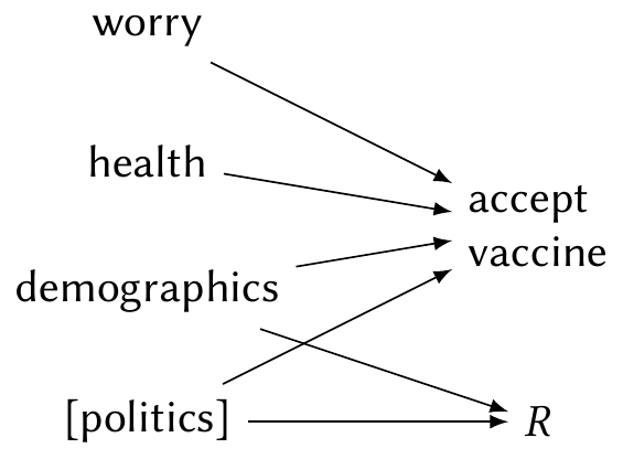
Because the missingness is not completely at random, but is also not dependent solely on observed variables, it is known as missingness not at random.
Definition 22.3 (Missing not at random) A variable \(X\) is missing not at random (MNAR) if it is neither missing completely at random (MCAR) nor missing at random (MAR). When a variable is MNAR, its probability of being missing may depend on a variable that is itself sometimes missing, or on a variable that is not observed at all.
MNAR is the most difficult case to deal with, because we cannot simply control for variables relating to missingness. The severity of the problem depends heavily on the exact structure of the missingness.
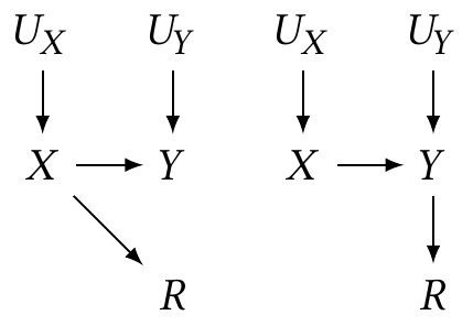
Example 22.1 (Two MNAR cases) Consider two possible cases. In each, \(R\) indicates missingness in \(Y\), but the mechanism is different:
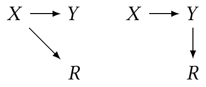
In the left-hand case, \(Y\) is missing based on the value of \(X\); in the right-hand case, \(Y\) is missing based on the value of \(Y\) (which is caused by \(X\)). Figure 22.4 plots these two scenarios in the case where the relationship between \(X\) and \(Y\) is linear. We can see that in the left case, conditioning on \(R = 1\) (using only complete cases) produces an unbiased estimate, while in the right case, conditioning on \(R = 1\) underestimates the slope.
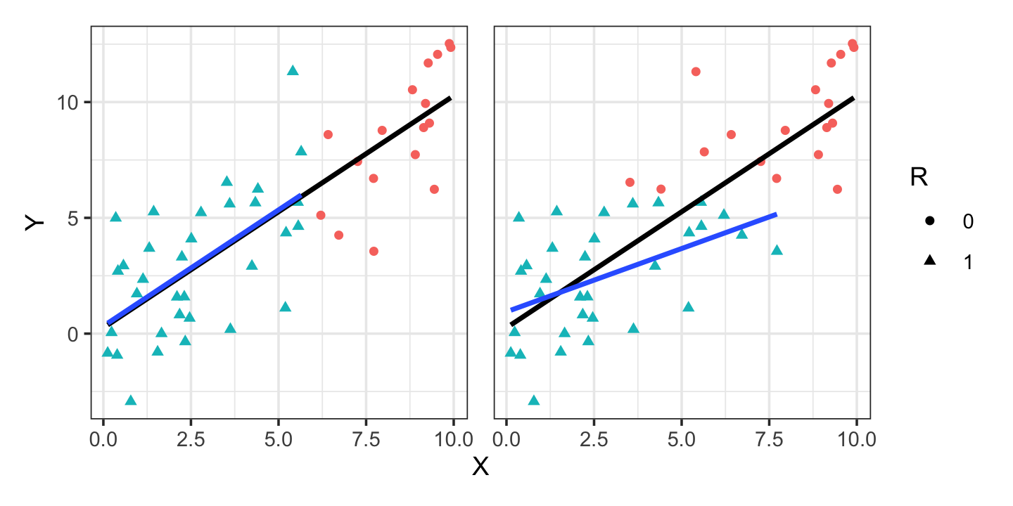
The plots suggest an intuitive explanation for the bias. In the first case, for any value of \(X\), we observe either the complete distribution of \(Y \mid X\) or nothing at all. We can hence estimate \(\E[Y \mid X = x]\), at least on the observed range of \(X\). (Obviously, if the relationship changes outside that range, we cannot extrapolate correctly.) But in the second case, for some values of \(X\) we do not observe the complete distribution of \(Y \mid X\), as it is truncated: \(Y\) is missing when it is too large.
To determine in which situations we can use a complete-cases analysis, we will need a way to assess the effect of conditioning on \(R\) given a causal diagram for the missingness. When a complete cases analysis would be biased, we may be able to model or predict the missing variables from the available data, allowing us to impute the missing data and then use it in our analysis. As we will see in Section 22.4, this can be done while accounting for uncertainty in the imputation, but it is difficult to tell if we have imputed accurately.
22.2 Judging the suitability of complete-cases analysis
To assess the effect of conditioning on \(R\)—that is, doing a complete-cases analysis—it is tempting to try to apply d-separation (Definition 2.3) directly. If conditioning on \(R\) opens up new non-causal paths, it introduces unwanted association; if it does not, then we can still estimate the desired \(X \to Y\) path.
That is not quite right, however. In Example 22.1, there is only one path from \(X\) to \(Y\), and conditioning on \(R\) doesn’t seem to open any other paths—and yet in one case, doing so causes us to estimate the wrong relationship. This is because we estimate relationships by applying the adjustment formula via regression (Section 2.4), and the adjustment formula applies only when the backdoor criterion is satisfied. And the backdoor criterion (Definition 2.4) requires that we do not condition on any descendant of \(X\). If \(R\) is a descendant of \(X\), such as in MAR or MNAR, the adjustment formula does not apply automatically.
We thus need an extension of the backdoor criterion that can work in these cases and tell us when we can or cannot use the adjustment formula. Using the unobserved error terms, Daniel et al. (2012) derived a procedure using to judge whether complete-cases analysis can be used to estimate causal effects. Their procedure extends the backdoor criterion (Definition 2.4) to create the generalized backdoor criterion.
Definition 22.4 (Generalized backdoor criterion) To determine whether the generalized backdoor criterion for the causal effect of \(X\) on \(Y\) is satisfied, draw a causal diagram for the problem. Include a node \(R\) representing completeness. Add nodes representing (potentially unobserved) parents of \(X\) and its descendants (except \(R\)). Let \(\condset\) be the set of variables we are conditioning on (controlling for). Then:
- Draw a dashed line between any pair of variables that are both parents of \(R\) or that share a child that is an ancestor of \(R\). These lines represent association induced by conditioning on \(R = 1\).
- Draw a dashed line between any pair of variables that are both parents of a variable in \(\condset\) or that share a child that is an ancestor of a variable in \(\condset\). These lines represent association induced by conditioning on \(\condset\).
Now consider every path (consisting of arrows in either direction and of dashed lines) from \(X\) to \(Y\), not passing through \(R\), that either starts with an arrow into \(X\) or contains a dashed line. Check whether each such path
- contains a collider, or
- passes through a variable in \(\condset\).
If the conditions are met for every path, the generalized backdoor criterion is satisfied.
Theorem 22.1 (Causal identification using complete cases) To estimate the causal effect of \(X\) on \(Y\) when conditioning on \(\condset\), the estimate based on complete cases (\(R = 1\)) is unbiased when
- the generalized backdoor criterion is satisfied, and
- all paths from \(R\) to \(Y\) are blocked by \(\condset\) or \(X\) (not counting paths with arrows into \(X\)).
Proof. See the Web Appendix of Daniel et al. (2012).
This is a complex set of conditions, so some examples may help.
Example 22.2 (Complete cases on the MNAR cases) Consider the two examples of Example 22.1. To apply the generalized backdoor criterion, we must modify the graphs by adding the unobserved parents of \(X\) and its descendants.
In the first example, when applying the backdoor criterion,
- There are no pairs of variables that are both parents of \(R\) or that share a child that is an ancestor of \(R\)
- We are not conditioning on any control variables, so \(\condset = \emptyset\).
Hence we draw no dashed lines. No path from \(X \to Y\) starts with an arrow into \(X\) or contains a dashed line, so the generalized backdoor conditions are trivially met. Using only the complete cases will be unbiased.
In the second example, when applying the backdoor criterion,
- \(X\) and \(U_Y\) share a child (\(Y\)) that is an ancestor of \(R\), so we must draw a dashed line between them. This represents the association between \(X\) and \(U_Y\) induced by using only the complete data: depending on the value of \(X\), we only observe \(Y\) if its noise source \(U_Y\) has a value that results in \(Y\) being observed.
- We are not conditioning on any control variables, so \(\condset = \emptyset\).
Now there is a path from \(X\) to \(Y\) containing a dashed line: \(X - U_Y \to Y\). It does not contain a collider or a variable in \(\condset\) (since \(\condset = \emptyset\)), so the path is open. The generalized backdoor criterion is not satisfied.
We have proved what the plots in Example 22.1 suggest: we can use a complete cases analysis in the first example, but in the second it would lead to a biased estimate of the \(X \to Y\) effect.
To summarize, then, we can use a complete-cases analysis when the conditions of Theorem 22.1 are met. These conditions are trivially met when the missingness is completely at random (Definition 22.1), as then there is no path from \(R\) to the rest of the causal graph. When the data is missing at random (Definition 22.2), if our control variables \(\condset\) contain all the variables affecting missingness (with arrows to \(R\)), we can use a complete cases analysis because \(\condset\) blocks any induced path in the generalized backdoor criterion. In any other case, we must carefully consider the situation to determine if a complete cases analysis is suitable. That consideration is difficult because parts of our causal graph are not testable: when a variable is missing, we cannot test if it is independent of other variables. Any analysis of missing data hence rests on untestable assumptions.
TODO Mohan and Pearl (2021)?
22.3 Completely missing cases and sampling bias
TODO sampling bias
The methods above have considered missingness in specific variables, but it is often the case that entire records are missing. In a survey, for example, we might invite a random sample of the relevant population to participate, but only some of those people will actually take the survey. What if their probability of participation is related to our variables of interest? We may obtain a biased sample, and in fact we can apply all the methods discussed above to describe this situation.
22.4 Imputation
While a complete case analysis can be suitable in some missing data situations, it may not be desirable: if a large fraction of data is missing, a complete case analysis may throw away most of the observations, resulting in high-variance estimates. In imputation, we keep the incomplete cases, using their observed data and imputing the missing variables.
There are several simple imputation strategies, though simple does not always mean wise. A common one is mean imputation: if a variable is missing, impute its value as the mean of the observed values. This is very easy to do, and seems “unbiased” in the sense that it assumes anything missing is average. But consider Figure 22.5, which imputes the missing data in Example 22.1 with its mean: the mean imputation seriously distorts the observed relationship between \(X\) and \(Y\), biasing our regression coefficients.
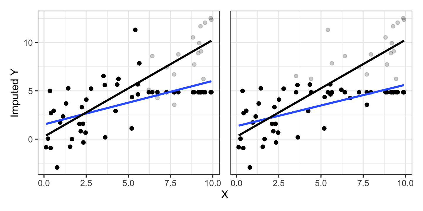
The bias arises because we want to estimate \(\E[Y \mid X = x]\), but have imputed missing values with \(\E[Y]\) alone. It would be better to impute missing values with something we believe respects the conditional relationship.
In data observed over time, such as time series data, a “last value carried forward” rule can be applied: if a measurement is missing at one time, assume it has the previously observed value. For example, if patients in a medical study have tests conducted every week, and a patient misses one week, we could carry their past test result forward to that week. This can be reasonable, as we’d expect the expected value for a patient this week to be close to their value last week, though it can still introduce bias in some circumstances; see Exercise 22.2.
More generally, we could use a model to impute the missing value by predicting it from the observed values. If our research goal is to estimate the regression model \[ Y = \beta_0 + \beta_1 X_1 + \beta_2 X_2 + e, \] but \(X_2\) is missing at random, we could fit a separate regression model to predict \(X_2\) using \(X_1\). We could then use the model to estimate the missing values of \(X_2\), and use those in our final regression.
This is called single imputation, as it replaces each missing value with a single estimate. Mean imputation is a special case where the imputation model only has an intercept. If \(X_2\) is missing at random, meaning its missingness is random conditional on the observed covariates, the regression of \(X_2\) on \(X_1\) using complete cases will be unbiased, so the procedure is valid—though while the imputed values may be unbiased, there is no guarantee that \(X_1\) strongly predicts \(X_2\)!
That suggests we need some way of accounting for the uncertainty in the process. If \(X_1\) strongly predicts \(X_2\), meaning the imputed values are very close to the true missing values, our final regression will be very good, but the sampling distribution of \(\hat \beta\) will be wider than normal, as each new sample would also lead us to fit a different model for imputation. If \(X_1\) is only a weak predictor of \(X_2\), the imputed values may be far from the truth, and our final inference for \(\beta\) should account for this.
22.4.1 Multiple imputation
The solution is multiple imputation. In multiple imputation, we refit our model several times with different imputed values, obtaining multiple estimates. This allows us to estimate the uncertainty in the imputation and estimation process.
Definition 22.5 (Multiple imputation) Consider fitting the model \[ Y = \beta_0 + \beta_o\T X_o + \beta_m\T X_m + e, \] where \(X_o\) is a vector of observed covariates and \(X_m\) is a vector of covariates that are missing at random. Let \(\beta = (\beta_0, \beta_o, \beta_m)\) be the complete parameter vector. In multiple imputation, we:
- Estimate the conditional distribution of \(X_m\) given \(X_o\) using the complete cases.
- For each missing value, draw a value from \(X_m \mid X_o\) given its observed covariates.
- TODO
22.4.2 MICE
TODO
Buuren and Groothuis-Oudshoorn (2011)
Exercises
Exercise 22.1 (Applying the generalized backdoor criterion) Apply the generalized backdoor criterion (Definition 22.4) to the CTIS situation in Figure 22.3, for the relationship between demographics and vaccine acceptance. Draw the augmented causal diagram and state whether the criterion is satisfied.
Exercise 22.2 (Last value carried forward) TODO last-carried-forward and regression to the mean (Gelman et al. (2021), p 325)
maybe simulate it and show the regression to the mean?