lambdas <- c(1e-5, 1e-4, 1e-3)
fits <- lapply(lambdas, function(lambda) {
  smooth.spline(doppler_samp$x, doppler_samp$y, lambda = lambda)
})14 Generalized Additive Models
\[ \DeclareMathOperator{\E}{\mathbb{E}} \DeclareMathOperator{\R}{\mathbb{R}} \DeclareMathOperator{\RSS}{RSS} \DeclareMathOperator{\AIC}{AIC} \DeclareMathOperator{\bias}{bias} \DeclareMathOperator{\MSE}{MSE} \DeclareMathOperator{\VIF}{VIF} \DeclareMathOperator{\var}{Var} \DeclareMathOperator{\cov}{Cov} \DeclareMathOperator{\cor}{Cor} \DeclareMathOperator{\se}{se} \DeclareMathOperator{\trace}{trace} \DeclareMathOperator{\vspan}{span} \DeclareMathOperator{\proj}{proj} \newcommand{\condset}{\mathcal{Z}} \DeclareMathOperator{\cdo}{do} \newcommand{\ind}{\mathbb{I}} \newcommand{\T}{^\mathsf{T}} \newcommand{\X}{\mathbf{X}} \newcommand{\Y}{\mathbf{Y}} \newcommand{\Z}{\mathbf{Z}} \newcommand{\zerovec}{\mathbf{0}} \newcommand{\onevec}{\mathbf{1}} \newcommand{\trainset}{\mathcal{T}} \DeclareMathOperator*{\argmin}{arg\,min} \DeclareMathOperator*{\argmax}{arg\,max} \DeclareMathOperator{\SD}{SD} \newcommand{\dif}{\mathop{\mathrm{d}\!}} \newcommand{\convd}{\xrightarrow{\mathrm{D}}} \DeclareMathOperator{\logit}{logit} \newcommand{\ilogit}{\logit^{-1}} \DeclareMathOperator{\odds}{odds} \DeclareMathOperator{\dev}{Dev} \DeclareMathOperator{\sign}{sign} \DeclareMathOperator{\normal}{Normal} \DeclareMathOperator{\binomial}{Binomial} \DeclareMathOperator{\bernoulli}{Bernoulli} \DeclareMathOperator{\poisson}{Poisson} \DeclareMathOperator{\multinomial}{Multinomial} \DeclareMathOperator{\uniform}{Uniform} \DeclareMathOperator{\edf}{edf} \]
Note
This chapter is based partly on notes cowritten with Ann Lee and Mark Schervish for 36-402, themselves based in part by notes by Cosma Shalizi.
Up until now, we’ve considered models that specify a particular parametric relationship between \(X\) and \(Y\). We have some more flexible parametric models, such as polynomials and splines (Chapter 10), but these are still limited in their flexibility, or require us to choose various tuning parameters (like the number and location of knots).
Ideally, we could say that our model is \[ Y = f(X) + e, \] for \(X \in \R^p\); for, for a generalized linear model, we’d like to say \[ Y \mid X = x \sim \operatorname{ExpFam}(f(x)), \] where ExpFam is some exponential dispersion family distribution (Definition 13.1). In both cases, we’d like as few restrictions on \(f\) as possible.
Unfortunately, estimating a general function \(f : \R^p \to \R\) with few restrictions is quite difficult, for two reasons:
- If we allow \(f\) to be arbitrarily complicated, without assumptions of linearity and without requiring the effect of different covariates be separable, we need a high density of observed points in order to estimate \(\hat f\). But the volume of \(p\)-dimensional space increases exponentially with \(p\), so the number of observations required to get a particular density (and hence fit with particular accuracy) increases exponentially with \(p\). This is the curse of dimensionality, and we will discuss it further in Chapter 16 when we quantify how well models fit.
- It is very hard to interpret \(\hat f\). How do you explain the association between, say, \(X_3\) and \(Y\), when the shape of \(f\) can be extremely complicated?
Fortunately, in many situations we are willing to make a basic assumption about \(f\): that it is additive. An additive model says that \[ Y = \beta_0 + f_1(X_1) + f_2(X_2) + \dots + f_p(X_p) + e, \] or sometimes \[ Y = \beta_0 + f_1(X_1) + f_2(X_2) + \dots + f_p(X_p) + f_{1,2}(X_1, X_2) + \dots + e. \] Each of the functions \(f_j\) can still be flexible and complicated, but the overall relationship is additive: it’s a sum of individual low-dimensional terms. We can write an analogous model for GLMs, as we will see in Section 14.3. First, let’s consider suitably flexible functions to use as the additive pieces.
14.1 Smoothers
In general, we can use any suitably flexible function that we have a procedure for fitting to data. In practice, we will prefer linear smoothers, which have some useful properties for inference.
Definition 14.1 (Linear smoothers) Consider a regression model for \(Y = r(X) + e\), fitting a function \(\hat r\) so that \(\hat Y = \hat r(X)\). A linear smoother is a regression estimator such that \[ \hat \Y = S \Y, \] for a matrix \(S\).
For example, ordinary least squares is a linear smoother, because \[ \hat \Y = \underbrace{\X (\X\T \X)^{-1} \X\T}_S \Y. \]
But we’re trying to find more flexible models, so let’s consider more flexible smoothers.
14.1.1 Univariate smoothers
Our experience with regression splines (Section 10.2) suggests they may be a useful and flexible smoother, apart from the need to choose knots. We can eliminate the need to choose knots by using a smoothing spline, motivated by the following result.
Theorem 14.1 (Smoothing splines) Consider data observed from a univariate regression model \(Y = r(X) + e\), and consider fitting a function \(\hat r(X)\) by minimizing the penalized sum of squares: \[ \hat r(x) = \argmin_{r(x)} \sum_{i=1}^n (Y_i - r(X_i))^2 + \lambda \int (r''(x))^2 \dif x. \] The penalty term penalizes curvature in the regression function. We can think of this as balancing the accuracy of the fit and the flexibility of the function, with the balance set by the tuning parameter \(\lambda > 0\), which must be fixed in advance.
The optimal function \(\hat r(x)\) will be a natural cubic spline with knots at each observed data point \(X_i\). This estimator is called a smoothing spline.
Proof. Wood (2017), section 5.1.1.
This gives motivation for the choice of a spline with one knot per observation (in univariate regression). It does not, however, tell us how to fit such a spline, or how to choose \(\lambda\). The theorem does not say that the solution is the same as the natural spline fit you would obtain by choosing one knot per observation and repeating the methods in Section 10.2 to fit; it says the solution is a natural cubic spline, but not which natural cubic spline. Which natural cubic spline depends on the choice of \(\lambda\).
Fortunately, we can write the solution in terms of a (more straightforward) optimization problem. Let \(p\) be the dimension of the natural spline basis with one knot per observation, and let \(\X \in \R^{n \times p}\) be the data expanded into the spline basis. (Recall that in Example 10.4 we saw how to take a univariate function and turn it into a matrix with \(p = 4\) columns, representing a piecewise linear spline. We can do the same for a cubic natural spline.)
The spline is then defined by \[ \hat \beta = \argmin_\beta \|\Y - \X \beta\|_2^2 + \lambda \beta\T \Omega \beta, \] where \(\Omega\) is a matrix with entries \[ \Omega_{jk} = \int B_j''(x) B_k''(x) \dif x, \] and \(B_j\) is the \(j\)th spline basis function (in the columns of \(\X\)). The solution is \[ \hat \beta = (\X\T\X + \lambda \Omega)^{-1} \X\T \Y. \]
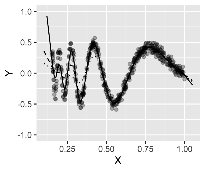
Example 14.1 (Smoothing spline for the Doppler function) In Example 10.6, we fit a natural spline to the Doppler function. Let’s try a smoothing spline instead, so we do not have to choose knots.
In R, we can use the smooth.spline() function to fit a univariate smoothing spline; it takes the \(X\) and \(Y\) observations as separate arguments. Let’s try a few values of \(\lambda\) to see their effect on the fit.
The fits are shown in Figure 14.1. The smaller values of \(\lambda\) are the most flexible, and the largest value gives the least flexible fit. Notice that all the fits become linear outside the range of the observed data, rather than diverging suddenly.
Of course, we have solved the problem of having to choose knots by introducing a new problem: the choice of \(\lambda\). But \(\lambda\) is a scalar, and in principle we can devise a procedure to try different values of \(\lambda\) and pick the one that produces the “best” fit. R will do this automatically if you allow it, and we’ll discuss procedures for estimating the error of fits in more detail in Chapter 17. For now it is sufficient to say that we will allow the value to be chosen automatically.
14.1.2 Multivariate smoothers
We can also define smoothers for functions of several variables. There are several ways to do this; see Wood (2017), sections 5.5 and 5.6, for full mathematical details. For our purposes, tensor product smoothers will be sufficient, and we will not get into the other methods.
Let’s motivate the basic idea by assuming we want to make a bivariate smoother \(f(y, z)\). Suppose we already have univariate smoothers that we can use to make univariate smoothers \(f_Y(y)\) and \(f_Z(z)\): \[\begin{align*} f_Y(y) &= \sum_{i=1}^I \alpha_i a_i(y)\\ f_Z(z) &= \sum_{j=1}^J \beta_j b_j(z). \end{align*}\] For example, these could be smoothing splines where \(a_i\) and \(b_j\) are the appropriate spline basis functions. How do we produce a smoother \(f_{YZ}\) that is bivariate? We could take \(f_Y\) and allow the coefficients to vary with \(Z\): \[ \alpha_i(z) = \sum_{l=1}^L \gamma_{il} b_l(z), \] reusing our basis functions \(b_l(z)\).
This gives the bivariate smoother \[ f_{YZ}(y, z) = \sum_{i=1}^I \sum_{l=1}^L \gamma_{il} b_l(z) a_i(y). \] This forms a sum of \(IL\) terms. We need only estimate \(\gamma_{IL}\). If we are using smoothing splines, \(I\) and \(L\) are determined by the number of unique values of each variable, and estimation can be done by defining a multivariate version of the smoothness penalty (Wood 2017, sec. 5.6.2).
This is called a tensor product smoother because the design matrix \(\X\) used to fit it can be written as a tensor product of the design matrices for \(f_Y\) and \(f_Z\). Consequently, if we have univariate smoothers, we can extend them to multivariate smoothers by using tensor products. The only danger is that the number of parameters to estimate is the product of the number of parameters for the individual smoothers.
14.1.3 Measuring smoothness
We need one more thing: a useful way to describe how flexible a particular smoother is, without referring to the penalty \(\lambda\). (We might also want to use a smoother other than splines, which may not have an equivalent to \(\lambda\).) For smoothing splines, \(\lambda\) is rather inconvenient because the size of the penalty depends on the range of \(X\): rescale \(X\) and a particular \(\lambda\) corresponds to a different amount of smoothness. This means it is not comparable between models or variables, so we need another way.
For a regression model with scalar outcome variable, we can instead define the effective degrees of freedom of each smoother.
Definition 14.2 (Effective degrees of freedom) When modeling \(Y = r(X) + e\), where \(\var(e) = \sigma^2\), the effective degrees of freedom (edf) of an estimator \(\hat r(x)\) is \[ \edf(\hat r) = \frac{1}{\sigma^2} \sum_{j=1}^n \cov(Y_j, \hat Y_j). \] Here \(X\) is fixed and the covariance treats \(Y\) as random, i.e., we obtain repeated samples of \(Y\) and measure the covariance between those samples and the new fitted values.
In matrix notation, this is \[ \edf(\hat r) = \frac{1}{\sigma^2} \trace \cov(\Y, \hat \Y). \]
We can show this is reasonable with some examples.
Example 14.2 (Intercept-only estimator) Consider fitting a model where \(\hat r(X)\) predicts just the intercept, i.e., \[ \hat Y = \frac{1}{n} \sum_{i=1}^n Y_i. \] Hence \[\begin{align*} \edf(\hat r) &= \frac{1}{\sigma^2} \sum_{i=1}^n \cov\left(\frac{1}{n} \sum_{j=1}^n Y_j, Y_i\right) \\ &= \frac{1}{\sigma^2} \sum_{i=1}^n \frac{1}{n} \var(Y_i)\\ &= 1, \end{align*}\] since the \(\cov(Y_j, Y_i) = 0\) for \(i \neq j\).
Example 14.3 (Linear regression estimator) Consider using linear regression, so that \(\hat \Y = \X(\X\T\X)^{-1} \X\T \Y\), where \(\X \in \R^{n \times p}\). Using the matrix form, \[\begin{align*} \edf(\hat r) &= \frac{1}{\sigma^2} \trace \cov(\X(\X\T\X)^{-1} \X\T \Y, \Y)\\ &= \frac{1}{\sigma^2} \trace \X(\X\T \X)^{-1} \X\T \cov(\Y, \Y) \\ &= \trace \X(\X\T \X)^{-1} \X\T \\ &= \trace \X\T\X (\X\T\X)^{-1}\\ &= \trace I\\ &= p. \end{align*}\] This follows because traces are invariant under cyclic permutations (Theorem 3.2) and because \(\X\T\X\) is a \(p \times p\) matrix, so we obtain the \(p \times p\) identity matrix, whose trace is the sum of \(p\) entries of 1 on the diagonal.
This suggests why the edf is called the edf: It is essentially like the number of free parameters required to represent the function. In a smoothing spline, different choices of \(\lambda\) correspond to different values of the edf, representing different amounts of smoothness; but unlike \(\lambda\), the edf is comparable between models and variables.
14.2 Additive models
This brings us back to additive models. An additive model says that \[ Y = \beta_0 + f_1(X_1) + f_2(X_2) + \dots + f_p(X_p) + f_{1,2}(X_1, X_2) + \dots + e, \] where \(f_1, \dots, f_p\) are smoothers, and multivariate smoothers such as \(f_{1,2}\) are added as desired. Just as univariate smoothing splines can be fit by a penalized form of least squares, so can additive models composed of smoothing splines (Wood 2017, sec. 4.3.2).
As written, the model is not identifiable: there are infinitely many combinations of the functions \(f_1, \dots, f_p\) that yield identical fits, because we can add and remove constants from each function. Typically we avoid this by imposing the constraint that \[ \sum_{i=1}^n f_j(x_i) = 0 \] for \(j = 1, \dots, p\). Similar constraints are applied to any multivariate smoother term. (This is much like ensuring identifiability when we have factors, as we saw in Section 7.4, where we had to impose a constraint on the factor coefficients.)
In R, the mgcv package provides all the tools necessary to fit additive models of arbitrary complexity, including automatically selecting the smoothness tuning parameters to achieve the best fit. (Again, we will discuss the types of procedures it uses in Chapter 17.) It reports the effective degrees of freedom for each spline term it fits; an edf of 1 corresponds to it choosing a linear relationship for that term. It also reports an approximate \(p\) value for each term, which you can think of as being approximately like an \(F\) test for the inclusion of that term, though the details are more complicated (Wood 2017, sec. 6.12.1).
Example 14.4 (Modeling wages) The ISLR package contains Wage, a data frame of data from a survey of incomes of men in the United States.
Let’s consider wages as a function of age, year, and education level. Age is in years; year is from 2003 to 2009; and education level is a factor variable representing different levels (from high school to advanced degrees). First let’s try a linear model and see if there’s any sign of nonlinearity.
library(ISLR)

wage_fit <- lm(wage ~ age + year + education, data = Wage)
The partial residuals are shown in Figure 14.2, and there does appear to be a nonlinear trend in age, particularly comparing the 20–40 and 40–60 trends.

To fit an additive model, we’ll load mgcv. It has a gam() function that takes a formula, and that formula can contain s() terms that represent smoothing splines. We’ll include a spline term for year as well, so we can check later if it is necessary; because there are only 7 years in the data, we will tell s() to only consider splines with fewer effective degrees of freedom. Notice that we can include education without s() because it is a factor; any term without s() will be treated just like it would be in a linear model or GLM.
library(mgcv)

additive_fit <- gam(wage ~ s(age) + s(year, k = 6) + education,
                    data = Wage)
summary(additive_fit)
Family: gaussian
Link function: identity

Formula:
wage ~ s(age) + s(year, k = 6) + education

Parametric coefficients:
                            Estimate Std. Error t value Pr(>|t|)
(Intercept)                   85.441      2.152  39.698  < 2e-16 ***
education2. HS Grad           10.984      2.428   4.524 6.31e-06 ***
education3. Some College      23.534      2.557   9.202  < 2e-16 ***
education4. College Grad      38.197      2.542  15.025  < 2e-16 ***
education5. Advanced Degree   62.585      2.759  22.688  < 2e-16 ***
---
Signif. codes:  0 '***' 0.001 '**' 0.01 '*' 0.05 '.' 0.1 ' ' 1

Approximate significance of smooth terms:
          edf Ref.df     F  p-value
s(age)  4.857  5.930 38.12  < 2e-16 ***
s(year) 1.147  1.278 10.43 0.000432 ***
---
Signif. codes:  0 '***' 0.001 '**' 0.01 '*' 0.05 '.' 0.1 ' ' 1

R-sq.(adj) =   0.29   Deviance explained = 29.3%
GCV = 1240.2  Scale est. = 1235.7    n = 3000
Here we can see that gam() has automatically chosen the penalty parameters, and has also fit separate intercepts for each level of education. It reports the edf it chose for each smoother: age has a more flexible smoother function than year, which has a nearly linear (edf nearly 1) smoother.
The plot() method for gam() fits will automatically plot each smoother term, as shown in Figure 14.3. The dashed lines indicate 95% confidence intervals. (Actually these are Bayesian credible intervals that happen to have good frequentist coverage; see Wood (2017), section 6.10.)
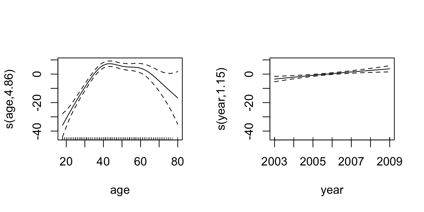
gam() to the wage data.
Notice both of these plots are centered around \(Y = 0\), due to the identifiability constraint imposed during fitting.
As shown above, additive models are sums of multiple terms, potentially including multivariate terms. These allow interactions between regressors. There are two ways to do this:
- For the interaction between a continuous predictor and a factor, fit a separate smoother to the continuous predictor for each factor level.
- For interactions between two or more continuous predictors, use multivariate smoothers (Section 14.1.2).
Example 14.5 (Modeling wages with interactions) Continuing from Example 14.4, consider allowing an interaction between age and education level. The s() function in mgcv takes a by = argument that fits a separate smoothing spline for each level of the factor, as shown below. The resulting spline fits are shown in Figure 14.4.
int_fit <- gam(wage ~ year + s(age, by = education),
               data = Wage)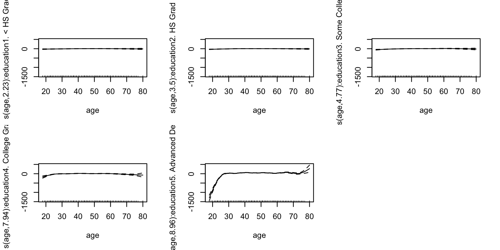
gam(), one for each education level.
To fit a bivariate term including both age and year, we can use either te() or ti() in the model formula. te() represents a tensor product smooth, so we could fit a model with:
te_fit <- gam(wage ~ te(age, year) + education,
              data = Wage)
Alternately, we could try to decompose the smooth into main effects and an interaction, just like in linear regression. ti() calculates the right basis to do this:
ti_fit <- gam(wage ~ s(age) + s(year, k = 6) +
                ti(age, year) + education,
              data = Wage)
summary(ti_fit)
Family: gaussian
Link function: identity

Formula:
wage ~ s(age) + s(year, k = 6) + ti(age, year) + education

Parametric coefficients:
                            Estimate Std. Error t value Pr(>|t|)
(Intercept)                   85.373      2.156  39.606  < 2e-16 ***
education2. HS Grad           11.160      2.432   4.589 4.64e-06 ***
education3. Some College      23.645      2.561   9.231  < 2e-16 ***
education4. College Grad      38.267      2.545  15.038  < 2e-16 ***
education5. Advanced Degree   62.688      2.761  22.701  < 2e-16 ***
---
Signif. codes:  0 '***' 0.001 '**' 0.01 '*' 0.05 '.' 0.1 ' ' 1

Approximate significance of smooth terms:
               edf Ref.df      F p-value
s(age)       4.930  5.997 37.981 < 2e-16 ***
s(year)      1.102  1.196 11.649 0.00028 ***
ti(age,year) 3.263  4.380  0.885 0.45087
---
Signif. codes:  0 '***' 0.001 '**' 0.01 '*' 0.05 '.' 0.1 ' ' 1

R-sq.(adj) =  0.291   Deviance explained = 29.4%
GCV = 1240.3  Scale est. = 1234.4    n = 3000
Notice that mgcv has calculated hypothesis tests for the smooth terms; these are roughly the equivalent of an \(F\) test for dropping each term, and evidently the bivariate term does not appear to be necessary here. We’ll discuss these tests further in Section 14.4.
14.3 Generalized additive models
The relationship between additive models and generalized additive models (GAMs) is much like the relationship between linear models and generalized linear models. In a GAM, we model \[ g(\E[Y \mid X = x]) = \beta_0 + f_1(x_1) + f_2(x_2) + \dots + f_p(x_p), \] where \(Y\) has an exponential dispersion family distribution, \(g\) is a link function, and \(f_1, \dots, f_p\) are smoothers. Multivariate smoothers can be used as well.
Just like in additive models with spline smoothers, where we could fit the model with a penalized form of least squares, we can fit GAMs with spline smoothers using a penalized version of maximum likelihood. This can be done iteratively in a procedure that looks much like IRLS. See Wood (2017), section 4.4 and chapter 6, if you want to know technical details.
Example 14.6 (Spam detection) This example comes from Hastie et al. (2009), chapter 9. It covers several thousand emails collected in the late 1990s at HP Labs. Each email had 57 features extracted, and our goal is to classify the emails as spam or not spam.
The data is provided from the UCI Machine Learning Repository as a CSV, which I have adapted to contain proper column names. The first 48 columns are the frequencies (percentages) of words in each email that are specific words, such as “business” or “credit” or “free”. The next 6 columns cound the frequencies of specific characters. The next few columns look at capitalization in the email, and the last column indicates if the email was spam (1) or not (0).
spam <- read.csv("data/gam-spam.csv")First, let’s make an ordinary logistic regression model as a baseline. We predict spam status using a few columns that we might guess are related to spam:
logistic_fit <- glm(spam ~ word_freq_make + word_freq_free +
                      word_freq_credit + word_freq_meeting,
                    data = spam, family = binomial())
Warning: glm.fit: fitted probabilities numerically 0 or 1 occurredWe get a warning: what does this mean?
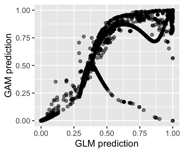
Let’s try the same with a generalized additive model. The gam() function accepts a family argument just like glm(). The hard part here is just making the model formula, since we want to write s() of every variable, and there are lots of them. Rather than writing this out by hand, we’ll paste together a formula:
gam_fit <- gam(spam ~ s(word_freq_make) + s(word_freq_free) +
                 s(word_freq_credit) + s(word_freq_meeting),
               data = spam, family = binomial())
We can get the predicted spam probabilities from both methods using predict(). Figure 14.5 shows that both models tend to predict probabilities near 0 and 1, but when they predict probabilities in between, they often disagree substantially.
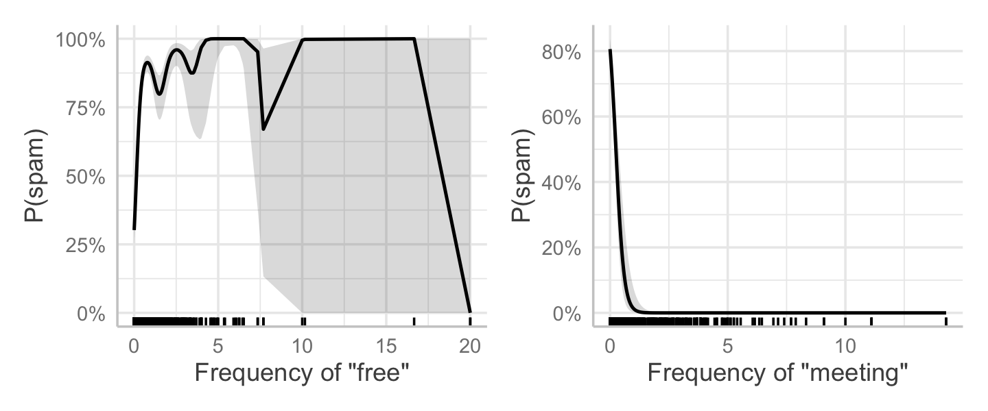
We can make effect plots in GAMs just like in any other regression. If we have no interaction terms (no terms involving two or more predictors), the effect plots vary \(X_j\) while holding the other predictors fixed at their means, and transform the result back to the response scale. For example, Figure 14.6 shows the plot for word_freq_free and word_freq_meeting. As the frequency of “free” increases, the probability of spam shoots up—though for large frequencies (more than 5–10 uses), there are very few emails in the data. On the other hand, it appears spam emails to not tend to talk about meetings, and the word “meeting” seems to correspond with a low probability of being spam.
Finally, it might be interesting to know how good our classifiers are. Can we make a decent spam filter based on just four features and a GAM? Let’s classify by marking as “spam” anything whose predicted probability is greater than 0.5. Table 14.1 shows the resulting confusion matrices, which suggest the GAM is better at detecting spam (more spam emails are correctly marked as spam), but also misclassifies ham emails as spam slightly more often than the logistic fit. Neither is a perfect classifier, but then we only used four predictors and made no effort to improve the models. (Also, if we want to evaluate the accuracy more fairly, we should use the methods we will discuss in Chapter 17.)
| Label |
GAM
|
Logistic
|
||
|---|---|---|---|---|
| Ham | Spam | Ham | Spam | |
| Ham | 2572 | 216 | 2639 | 149 |
| Spam | 689 | 1124 | 988 | 825 |
14.4 Inference and interpretation
In additive models, inference is more complicated than in the regression models we’ve discussed so far. With spline smoothers, there’s no convenient slope parameter to interpret, so we can’t simply quote a confidence interval for a slope to describe our results. Worse, if we allow mgcv to automatically select the penalty parameters, any inference procedure needs to account for the fact that on a new sample of data, we’d get different penalty parameters.
The mgcv package can produce tests for both linear terms (those without smoothers) and smooth terms. These are based on approximate results described in Wood (2017), section 6.12.
To compare multiple models fit with gam(), the package provides an anova() method. This performs a likelihood ratio test.
Confidence intervals on smoothed coefficients are likely not useful, but we may want confidence intervals for the fitted mean \(\E[Y \mid X = x]\). The predict() method for GAMs can give standard errors (by setting se.fit = TRUE), which can be used to construct an approximate normal confidence interval.
TODO more detail
Exercises
Exercise 14.1 (Shalizi (2026), assignment 12) The gamair package contains chicago, a data frame of air pollution data from Chicago, Illinois. (The package is old, so you have to use data(chicago) to get it to actually load the data; most newer R packages no longer require this.) Each row represents one day. The variables are:
- time: The date of observation, given as the number of days before or after December 31, 1993. (The
as.Date()function can convert this to a date by using theoriginargument to specify day 0.) - death: The number of non-accidental deaths in Chicago on that date
- pm10median: The median density of PM10 pollution, i.e., particulate matter with diameter less than 10 micrometers (milligrams per cubic meter). (The dataset also contains PM2.5 measurements, but a large fraction of these are missing, so we will not use them)
- o3median: The median concentration of ozone (parts per billion)
- so2median: The median concentration of sulfur dioxide (SO2)
- tmpd: The mean temperature (Fahrenheit)
Some of the pollution variables have been shifted, so they contain negative values.
The pollution and temperature variables also have versions whose names start with lag_. These versions are 7-day averages of the original variables; for example, lag_pm10median on day 7 is the average of pm10median on days 1 through 7. For this exercise, we will ignore the lagged variables.
A few observations contain NA values. You can ignore these observations.
We’d like to establish if there is evidence the pollution variables are associated with death rates, and if so, determine the form of the association. Given that the outcome variable (deaths) is a count of deaths, which response distribution makes sense to use here? Pick a distribution and use it for your models in the subsequent parts.
Conduct a brief exploratory data analysis for the relationships between the predictors and death rates. What associations do you see?
Consider three models, each with deaths as the outcome variable:
- Model 0: No predictors, only an intercept
- Model 1: Generalized linear model predicting death rates using the three pollution variables and temperature
- Model 2: Additive model version of Model 1, in which each term is a spline smoother
Fit these models to the data. Briefly conduct diagnostics to check their fits.
Note: In order to compare the models, it will be necessary for them to be fit to the same data. Because a few observations of the variables are missing, Model 1 and Model 2 will omit a few rows of data. Be sure to fit Model 0 to only the rows of data with the variables present, so it’s fit to the same data.
Finally, one substantive question is whether it’s pollution and temperature on their own that cause high death rates, or if it is their combination. Select a GAM that could help answer this question, fit it, and interpret your results.
Exercise 14.2 (Effective degrees of freedom of linear smoothers) Show that the effective degrees of freedom (Definition 14.2) for a linear smoother (Definition 14.1) can be written \[ \edf(\hat r) = \trace S, \] where \(S\) is the smoothing matrix and we assume the true relationship is \(Y = r(X) + e\), where the errors are independent with common variance \(\sigma^2\).