18 Penalized Models

When we were using regression for inference—to learn parameters of specific scientific interest—we wanted our models to be as close to the true population relationship as possible, and we chose unbiased estimators to ensure our parameter estimates would, on average, be unbiased. If the whole point of regression is to get a good \(\hat \beta\) to tells us something about the true population relationship, those seem like reasonable goals.

But if our goal is prediction, we might instead be interested in predicting with minimal error. And the bias-variance tradeoff (Section 16.3) says that total error is a combination of bias and variance—and the optimal combination might have nonzero bias. If we can reduce the variance in some meaningful way, perhaps we can get lower error despite using biased estimators for the model.

As a motivating example, consider using the model \[ Y = \beta\T X + e \] to predict \(Y \in \R\) from regressors \(X \in \R^p\). If we obtain a dataset of size \(n\), we know that we can use least squares to estimate \(\hat \beta\) and that it will be unbiased. But if we’re trying to make a predictive model, we might have collected a large number of predictors; and we might also consider nonlinear transformations of those predictors (Chapter 10), in case the relationship is nonlinear. Both of these may result in a large number of regressors, \(p\).

We know that adding useful predictors can reduce \(\var(e)\), improving our inference, and that if the true relationship is nonlinear, adding nonlinear regressors can reduce the bias of our model. On the other hand, we know that linear regression’s variance is proportional to \(p\). As the generalization error is the sum of the bias and the variance (Exercise 16.5), there is a tradeoff: adding regressors improves the fit by reducing the bias, but also increases the variance. Somehow we want to add the right regressors that reduce the bias, but not any useless ones that don’t.

One approach is to check each regressor’s usefulness when we add it. We could, for instance, use forward stepwise selection.

Definition 18.1 (Forward stepwise selection) Consider predicting \(Y\) from a set of possible predictors. Define the model scope to be the full set of regressors (derived from the predictors) that can be included in the selected model. Then:

Start with an empty model, i.e., one with only an intercept.
For each term in the scope that is not yet in the model, fit a model including that term.
Compare the new model to the previous model using some criterion (such as an \(F\) test, AIC, or Mallows’ \(C_p\)).
Select the term that improves the criterion the most (e.g., improves the AIC the most). Add it to the model.
Return to step 2 and repeat. Stop the process if no term improves the criterion enough.

For example, the model scope could be represented by the formula

Y ~ X1 + poly(X2, 3) + X3 + X4 + X3:X4

and on the first iteration, the model would choose whether to add regressors for X1, poly(X2, 3), X3, or X4. (Often the “marginality principle” of Section 7.5 is followed, where interactions are not considered unless the main effects are already in the model.)

But as we saw in Example 11.5 and Example 11.6, procedures like forward stepwise regression have an unfortunate property: the distribution of \(\hat \beta\) is much more complicated, because some coefficients are either zero (when that predictor is not included in the model) or nonzero (when it is) depending on the particular sample obtained from the population. Or, in other words, the inclusion or exclusion of a predictor from the model is a discrete event, resulting in a sampling distribution that is a mixture of different distributions for different combinations of included predictors. This increases the variance compared to a single model using only one particular subset of the predictors. (TODO Harrell, section 4.3) And as we saw in Example 17.3, stepwise selection can overfit easily, selecting “lucky” variables that have an association with \(Y\) even when there is no true signal.

There are other stepwise selection methods: backwards stepwise selection, for example, starts with a large model and sequentially considers terms to remove. But these all have similar limitations. They are known as greedy algorithms because they try to find an optimal solution (the best model) by sequentially taking the best decision at each step (which variable to add or remove); and like many greedy algorithms, they are not guaranteed to find a globally optimal solution.

18.1 Penalization

Penalization, also known as shrinkage or regularization, is another approach to reduce variance when we have many regressors. In penalized regression, our estimator includes the loss function but also a penalty: large values of \(\hat \beta\) are worse than smaller values. For instance, in linear regression, our estimator might be \[ \hat \beta = \argmin_\beta \frac{1}{2n} {\underbrace{\|\Y - \X \beta\|_2^2}_\text{error}} + {\underbrace{\lambda \|\beta\|}_\text{penalty}}, \] where \(\| \cdot \|\) is a norm (Definition 3.7). Picking different norms will result in different estimators with different useful properties, as we will see below. The parameter \(\lambda\) is a tuning parameter. Much like the penalty parameter in smoothing splines (Theorem 14.1), it controls the amount of penalization or the amount of shrinkage. When \(\lambda = 0\), we have the ordinary least squares fit; when \(\lambda\) is large, \(\hat \beta\) is penalized heavily. This results in \(\hat \beta\) being shrunken toward 0.

Generalized linear models are usually fit by maximum likelihood instead of by least squares (Section 13.2). We can apply a similar penalty to the maximum likelihood problem: \[ \hat \beta = \argmin_\beta -\frac{1}{n} {\underbrace{\ell(\beta)}_\text{likelihood}} + {\underbrace{\lambda \|\beta\|}_\text{penalty}}. \]

We can immediately see a few properties that will be shared by penalized regression methods:

The estimator \(\hat \beta\) is biased. It is not the ordinary least-squares or maximum likelihood estimate.
We will need to choose \(\lambda\). It is a tuning parameter, not something that can be estimated from the data as part of the fit. We will need additional steps, such as cross-validation, to choose the \(\lambda\) that produces the best fit for our purposes.
Scaling matters. In least squares regression, rescaling a column of \(\X\) by a constant will rescale the corresponding entry of \(\beta\), but otherwise does not change the fit (see Exercise 5.1). But here, rescaling a column of \(\X\) by a constant means the corresponding entry of \(\beta\) will be penalized more or less heavily. That may change the optimal solution and the predictions made by the model, so we will need a principled way to choose the “right” scaling of \(\X\).
Calculating \(\hat \beta\) from the optimization problem above may be nontrivial. We’ll see that for some choices of the norm \(\|\beta\|\), a solution can be obtained in closed form, but for others, an algorithm will be required to find the solution.
Estimating \(\var(\hat \beta)\), producing confidence intervals, or conducting hypothesis tests will also be more challenging in penalized methods, though this is usually not our goal anyway. The penalty will change the sampling distribution of \(\hat \beta\), potentially very substantially, depending on our choice of \(\lambda\).

18.1.1 Regressor scaling

As mentioned above, scaling matters in penalized regression. A model can have very different parameters depending on the scaling of its regressors: \[\begin{align*} \text{bill length (mm)} &= 14 + 0.13 \times \text{flipper length (mm)} + e\\ &= 14 + 3.3 \times \text{flipper length (in)} + e \\ &= 14 + 1.3 \times 10^5 \times \text{flipper length (km)} + e. \end{align*}\] Each of these would have very different values of \(\|\beta\|\) despite identical fits. When there are multiple regressors, each would be penalized according to its scale, so some regressors may have coefficients heavily shrunken towards 0 while others have coefficients that are hardly changed from the least-squares fit.

The intercept \(\beta_0\) is typically not penalized (it is left out of the norm \(\|\beta\|\)), since the intercept can be of arbitrary size depending on the range of \(X\) and \(Y\).

When regressors are on the same scale and it makes sense to penalize them equally, we may enter them as-is into the regression. When regressors are on different scales, it is common to standardize them by dividing by their standard deviation in the training sample, so each has variance 1. This is often automatically done by packages, and the estimated coefficients automatically transformed back to the original scale.

18.1.2 More complex regressors

In Chapter 10, we discussed allowing complex and nonlinear relationships between predictors and response variables by representing a predictor with multiple regressors. For example, we could allow a cubic polynomial relationship between \(X_1\) and \(Y\), or we could use a cubic spline by using the spline basis functions to generate regressors. In either case, there are many possible bases: with polynomials, we can use the regressors \(\{X_1, X_1^2, X_1^3\}\), or we can use an orthogonal polynomial basis; with splines, we can construct a basis as in Example 10.4 or use the B-spline basis. These choices result in different scales for the columns of \(\X\), and thus different magnitudes of \(\beta\); thus the fit of the penalized regression will depend on our choice of basis.

A similar issue affects factor predictors. As we saw in Section 7.4, there are multiple ways to encode factors in \(\X\), the most common of which (at least in R) is treatment contrasts (Definition 7.1). One factor level is absorbed into the intercept, and the regressors encode differences between that baseline level and the other levels. Consequently, shrinking \(\beta\) towards zero shrinks all factor levels toward the baseline level. Using a different baseline results in a different fit.

If the factor regressors are standardized, the amount of penalization also depends on the rate of occurrence of each factor level. Consider the simple case of a binary predictor, which enters as a regressor \(X_j \in \{0, 1\}\). Suppose the fraction of cases with \(X_j = 1\) is \(q\). The variance of \(X_j\) is hence \(q(1 - q)\), so the standardized regressor will be \(X_j^* \in \{0, 1/\sqrt{q(1 - q)}\}\). The scale of the regressor standardized depends on \(q\), so the magnitude of \(\beta_j\) depends on \(q\), and hence the amount of penalization applied to it.

For factors with more than two levels, this means each level will have a different amount of penalization, and a different amount of shrinkage toward the baseline level. This is conceptually unsatisfying. While it may be possible to fix by changing the standardization process (Larsson and Wallin 2025), in practice the problem is simply ignored, even though it may affect results in penalized regression where interpreting the factor variables is important.

18.2 Ridge regression

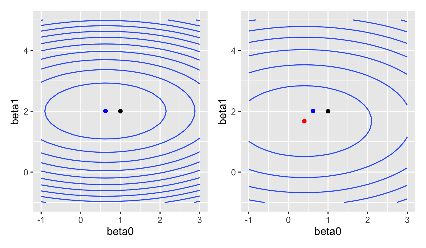
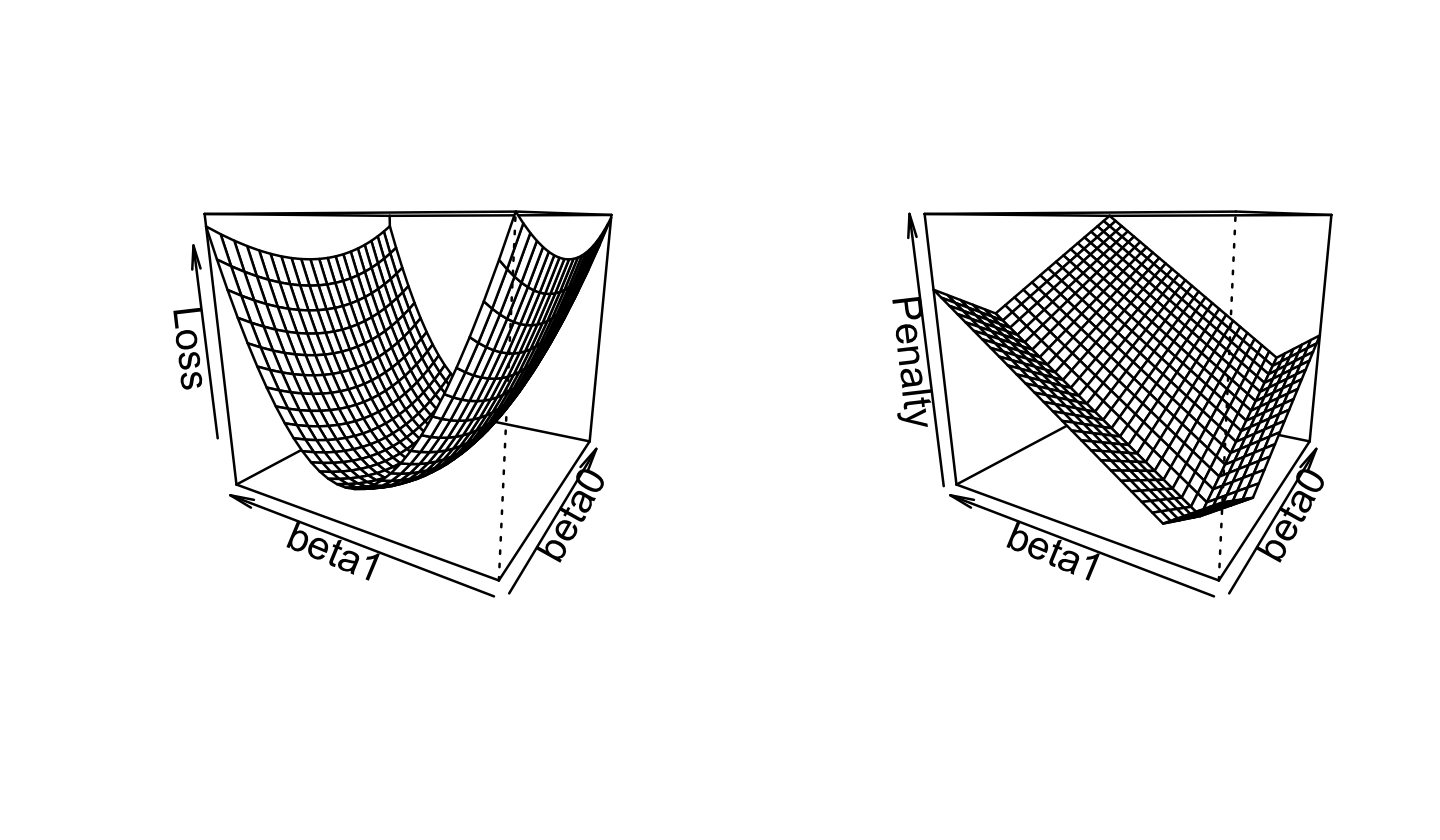
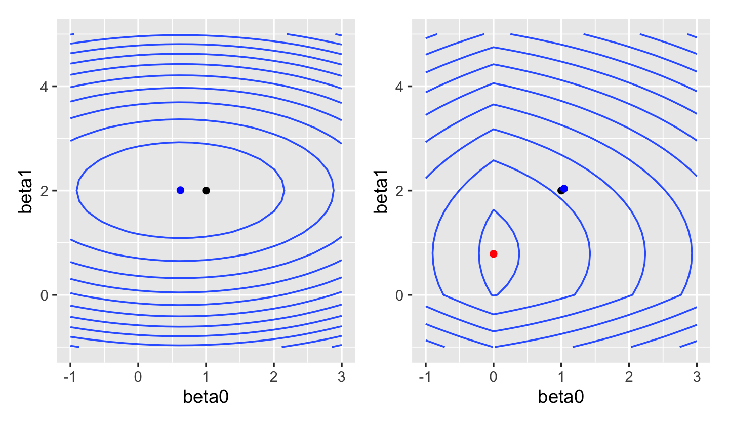
In ridge regression, we use the Euclidean norm (Definition 3.8) for the penalty term: \[ \hat \beta_\text{ridge} = \argmin_\beta \frac{1}{2n} {\underbrace{\|\Y - \X \beta\|_2^2}_\text{error}} + {\underbrace{\lambda \|\beta\|_2^2}_\text{penalty}}. \] The original squared-error loss was quadratic in \(\beta\), and this remains quadratic in \(\beta\). We can plot the squared-error loss as a function of \(\beta\) for a fixed dataset, as shown in Figure 18.1. If we compare this to the ridge loss, shown in Figure 18.2, we see the shape is fairly similar—but the optimal solution has shifted towards \(\hat \beta = \zerovec\).

Figure 18.1: The shape of the squared-error loss function for a simple linear regression problem, plotted against \(\beta_0\) and \(\beta_1\).

Figure 18.2: *Left:* Contours of the loss function shown in Figure 18.1, with the true \(\beta\) marked in black and the least-squares \(\hat \beta\) in blue. *Right:* Contours of the ridge regression loss function with \(\lambda = 4\), with the ridge \(\hat \beta\) marked in red. Notice the solution has shifted towards \((0, 0)\).

This optimization problem can also be written in a constrained form: \[\begin{align*} \hat \beta_\text{ridge} &= \argmin_\beta \frac{1}{2n} \|\Y - \X \beta\|_2^2\\ \text{such that } & \|\beta\|_2^2 \leq t, \end{align*}\] where \(t\) is a tuning parameter. (The penalized form is the constrained form with a Lagrange multiplier; see Boyd and Vandenberghe (2004), section 5.1.) There is a one-to-one relationship between values of \(\lambda\) and values of \(t\) that produce identical solutions.

Crucially, this optimization problem has a unique solution even if \(p > n\). The solution is available in closed form (Exercise 18.1): \[ \hat \beta_\text{ridge} = (\X\T\X + 2 n \lambda I)^{-1} \X\T \Y, \] where \(I\) is the \(p \times p\) identity matrix. The matrix \(\X\T\X + 2n \lambda I\) is invertible even if \(\X\T\X\) does not have full rank. This is why you hear of ridge regression being used in high-dimensional problems; “high-dimensional” means \(p\) is large relative to \(n\).

Example 18.1 (Ridge in a univariate example) It’s easier to understand ridge regression in a univariate example. Suppose our model is \(Y = \beta + e\), with no covariates. The optimization problem is \[ \hat \beta_\text{ridge} = \argmin_\beta \frac{1}{2n} \sum_{i=1}^n (y_i - \beta)^2 + \lambda \beta^2. \] If we minimize this by taking the derivative and setting it to zero, we obtain \[\begin{align*} 0 &= \sum_{i=1}^n -\frac{1}{n} (y_i - \hat \beta) + 2 \lambda \hat \beta\\ &= \hat \beta - \frac{1}{n} \sum_{i=1}^n y_i + 2 \lambda \hat \beta\\ &= (2 \lambda + 1) \hat \beta - \frac{1}{n} \sum_{i=1}^n y_i\\ \hat \beta &= \frac{\frac{1}{n}\sum_{i=1}^n y_i}{2\lambda + 1} = \frac{1}{n(2 \lambda + 1)} \sum_{i=1}^n y_i. \end{align*}\] When \(\lambda = 0\), the solution is simply the sample mean of \(Y\); as \(\lambda \to \infty\), \(\hat \beta_\text{ridge} \to 0\).

Alternately, we can think of ridge regression as adding \(\lambda/2n\) “fake” observations with \(Y = 0\). When \(\lambda = 1/2n\), for instance, the denominator is \(n + 1\), so there was one fake observation with \(Y = 0\). As \(\lambda\) grows, the real data is dominated by the fake data, and the estimate converges asymptotically to zero.

Similar arguments can be made when we have covariates with their own slopes: they also converge towards zero as \(\lambda\) grows, but do not become exactly zero until \(\lambda \to \infty\).

Though the closed-form solution is convenient (and it is similar to how we fit smoothing splines in Section 14.1.1), often we do not know the right \(\lambda\) in advance and instead want to fit the model with many values of \(\lambda\) so we can evaluate which is best. Packages for fitting ridge regression often use alternate algorithms that can find the solution path efficiently, meaning they estimate the function \(\hat \beta_\text{ridge}(\lambda)\) for a range of values of \(\lambda\). There are clever iterative algorithms that can do this more efficiently than repeatedly evaluating the closed-form solution for many values of \(\lambda\) (Friedman et al. 2010; Hastie et al. 2015).

Example 18.2 (Ridge regression with glmnet) The glmnet package implements ridge, lasso, and elastic net regression. As its name implies, it can fit penalized forms of any generalized linear model. It implements the elastic net penalty (to be discussed in Section 18.4), of which ridge regression is a special case.

Let’s illustrate the value of penalized regression by simulating a sparse population: there are 100 predictor variables, of which only 5 actually have an association with \(Y\). We will take a sample of just 90 observations, which is clearly not enough to fit a full model.

library(regressinator)
library(mvtnorm)

sparse_pop <- population(
  x = predictor(rmvnorm,
                mean = rep(0, 100),
                sigma = diag(100)),
  y = response(4 + 0.2 * x1 - 5 * x2 + x3 + 0.4 * x4 + 8 * x5,
               error_scale = 1)
)

sparse_samp <- sparse_pop |>
  sample_x(n = 90) |>
  sample_y()

We will use the glmnet() function to fit the model. Unlike most model functions we’ve used, glmnet() requires us to provide \(X\) as a matrix and \(Y\) as a vector of responses; we cannot simply provide a data frame and a formula. One way to produce the desired \(X\) matrix is with the R function model.matrix(), though glmnet also provides makeX() to do a similar task.

x <- model.matrix(~ . - 1 - y, data = sparse_samp)

This formula means the matrix should use all variables (.), but not include an intercept (- 1) or our response variable (- y). Now we can load glmnet and fit the model, setting alpha = 0 to get the ridge regression penalty:

library(glmnet)

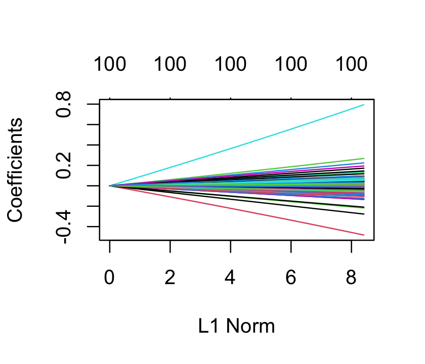
ridge_fit <- glmnet(x, sparse_samp$y, alpha = 0)

We did not have to standardize x, as glmnet() standardizes each column to have variance 1 automatically. Now ridge_fit represents not one fit but, by default, 100 fits with different penalty values. It has a plot() method that plots the coefficients as a function of the penalty, as shown in Figure 18.3. We can see that as the penalty parameter varies, the estimated coefficients shrink to zero.

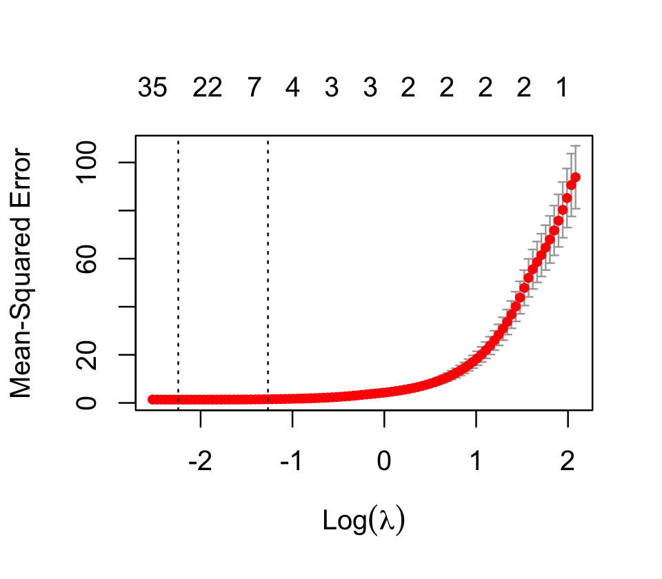
Figure 18.3: Solution paths for ridge regression. Each point on the \(X\) axis represents a ridge fit with a particular penalty parameter; here the \(X\) axis is labeled by the value of \(\|\hat \beta\|_1\) of each fit. Each line is one estimate \(\hat \beta_j\).

To pick one fit out of the many, we could use cross-validation, as described in Section 17.3. The cv.glmnet() function will automatically do \(k\)-fold cross-validation and return the penalty parameter with optimal error. By default, it does 10-fold cross-validation for every model, and returns all the estimated errors. It takes the data as arguments, as well as additional arguments passed on to glmnet() (such as alpha) to control the fits.

cv_results <- cv.glmnet(x, sparse_samp$y, alpha = 0)
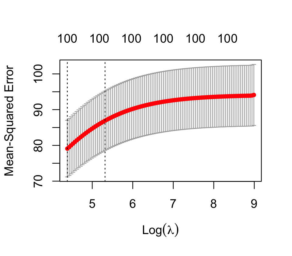
cv_results$lambda.min

[1] 89.33002

We can see that cross-validation has chosen \(\lambda = 89.3\) as the value that minimizes the error. There is also a plot() method for this object, producing the plot shown in Figure 18.4. Evidently this problem wants minimal regularization.

Figure 18.4: Ridge regression error (estimated by cross-validation) versus the log of the penalty parameter. The error bars indicate estimated standard errors.

Finally, we can get model coefficients or predictions by using coef() or predict(), as with most other models. These both take an argument s for the value of the penalty parameter for which coefficients or predictions are desired. For example, let’s see the parameter estimates with the largest magnitudes, and see if they match the predictors we know to have nonzero coefficients:

coefs <- coef(ridge_fit, s = cv_results$lambda.min)
coefs[order(abs(coefs[, 1]), decreasing = TRUE)[1:5], ]

(Intercept)          x5          x2         x70         x10 
  3.0092536   0.7245283  -0.4680285  -0.2396174   0.2177630

The intercept is very close to the true population value (4), and the ridge regression has pulled out \(X_2\) and \(X_5\) as two covariates with the largest estimates; but the other predictors, whose associations with \(Y\) have slopes smaller than 0.5, don’t appear in the top predictors. This is likely because, with 95 other predictors that have no association, the noise in their estimates is larger than the magnitude of the true effects for \(X_1\), \(X_3\), and \(X_4\).

Ridge regression is particularly valuable when there are collinear predictors. We saw in Section 9.5 that collinearity results in high prediction variance: in Example 9.9, a strong correlation between \(X_1\) and \(X_2\) meant predictions in part of the parameter space would have rapidly increasing variance. It also results in correlation between the affected components of \(\hat \beta\). But the ridge penalty reduces the covariance of \(\hat \beta\) by encouraging effects to be “shared” between collinear predictors, and as a result reduces the variance of predictions as well.

Example 18.3 (Collinearity in ridge regression) In Example 9.9, we considered a population where \(X_1\) and \(X_2\) were positively correlated, so in any particular sample they would be collinear:

library(regressinator)
library(mvtnorm)

collinear_pop <- population(
  x = predictor(rmvnorm,
                mean = c(0, 0),
                sigma = matrix(c(4, 3.75, 3.75, 4), ncol = 2)),
  y = response(
    4 + 2 * x1 - 3 * x2,
    family = gaussian(),
    error_scale = 1.0
  )
)

coll_sample <- collinear_pop |>
  sample_x(n = 100) |>
  sample_y()

We can fit a linear model to this data using ridge regression rather than least squares. As Figure 18.5 shows, as \(\lambda\) increases the loss function is less and less “stretched”. While in least-squares regression an increase in \(\hat \beta_1\) can be offset by a decrease in \(\hat \beta_2\), producing an almost identical fit, in ridge regression the magnitude of \(\hat \beta\) is penalized, making these solutions less favored.

Figure 18.5: Ridge regression loss for the collinear data with \(\lambda = 50\) (\(\hat \beta\) in blue) and \(\lambda = 500\) (\(\hat \beta\) in red). The true \(\beta\) is marked in black. As \(\lambda\) increases, the estimate shrinks towards 0, and the contours are much less stretched.

This tradeoff—of a biased \(\hat \beta\) versus lower prediction variance—is exactly the bias-variance tradeoff we discussed in Section 16.3. Often the best predictive model has \(\lambda > 0\), despite having nonzero bias.

18.3 The lasso

In the lasso, we use the Manhattan norm (Definition 3.9) for the penalty term: \[ \hat \beta_\text{lasso} = \argmin_\beta \frac{1}{2n} {\underbrace{\|\Y - \X \beta\|_2^2}_\text{error}} + {\underbrace{\lambda \|\beta\|_1}_\text{penalty}}. \] This optimization problem can again be written in a constrained form: \[\begin{align*} \hat \beta_\text{lasso} &= \argmin_\beta \frac{1}{2n} \|\Y - \X \beta\|_2^2\\ \text{such that } & \|\beta\|_1 \leq t, \end{align*}\] where \(t\) is a tuning parameter. There is a one-to-one relationship between values of \(\lambda\) and values of \(t\) that produce identical solutions. As with ridge regression, there is a unique \(\hat \beta_\text{lasso}\) even when \(p > n\), provided \(\lambda > 0\).

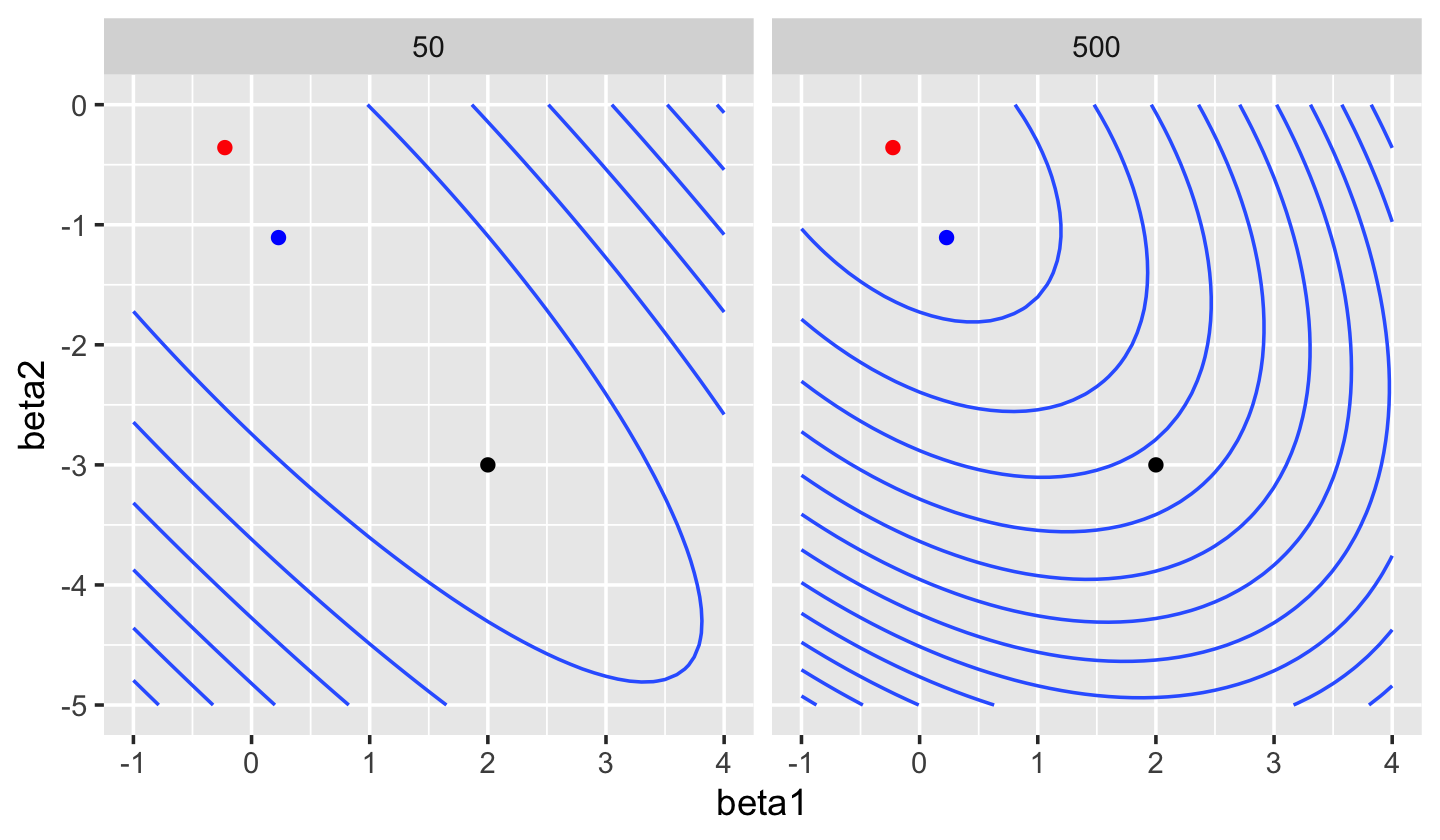
The lasso’s most useful property is that, depending on the value of \(\lambda\), it forces many entries in \(\hat \beta_\text{lasso}\) to be exactly zero. We can see this from the shape of the loss function in Figure 18.6: the penalty has a sharp corner when \(\beta_0 = 0\) or \(\beta_1 = 0\). When we plot the contours of the overall lasso loss function in Figure 18.7, we see this results in a loss with a valley along the \(\beta_0 = 0\) axis.

Figure 18.6: *Left:* The squared-error loss function. *Right:* The lasso penalty function. The discontinuities at \(\beta_0 = 0\) and \(\beta_1 = 0\) encourage sparsity.

Figure 18.7: *Left:* The squared-error loss contours, as in Figure 18.2. *Right:* The lasso loss contours when \(\lambda = 50\), with the squared-error estimator in blue and the lasso \(\hat \beta\) in red. Notice the discontinuities at \(\beta_0 = 0\) and \(\beta_1 = 0\).

If it’s hard to see why the penalty tends to make entries in \(\hat \beta_\text{lasso}\) exactly zero, let’s look at its shape in a simple case.

Example 18.4 (Different penalties) Suppose our model is \(Y = \beta + e\), so there is only one parameter, as in Example 18.1. The least-squares solution is \[\begin{align*} \hat \beta &= \argmin_\beta \sum_{i=1}^n (y_i - \beta)^2\\ &= \argmin_\beta \sum_{i=1}^n (y_i^2 - 2 \beta y_i + \beta^2). \end{align*}\] This is a quadratic in \(\beta\). If we take the derivative with respect to \(\beta\) and set it to zero, we get \[ \hat \beta = \frac{1}{n} \sum_{i=1}^n y_i. \]

Let’s suppose that \(\hat \beta=2\), and let’s consider what happens when we add \(L^1\) and \(L^2\) penalties, as shown in Figure 18.8.

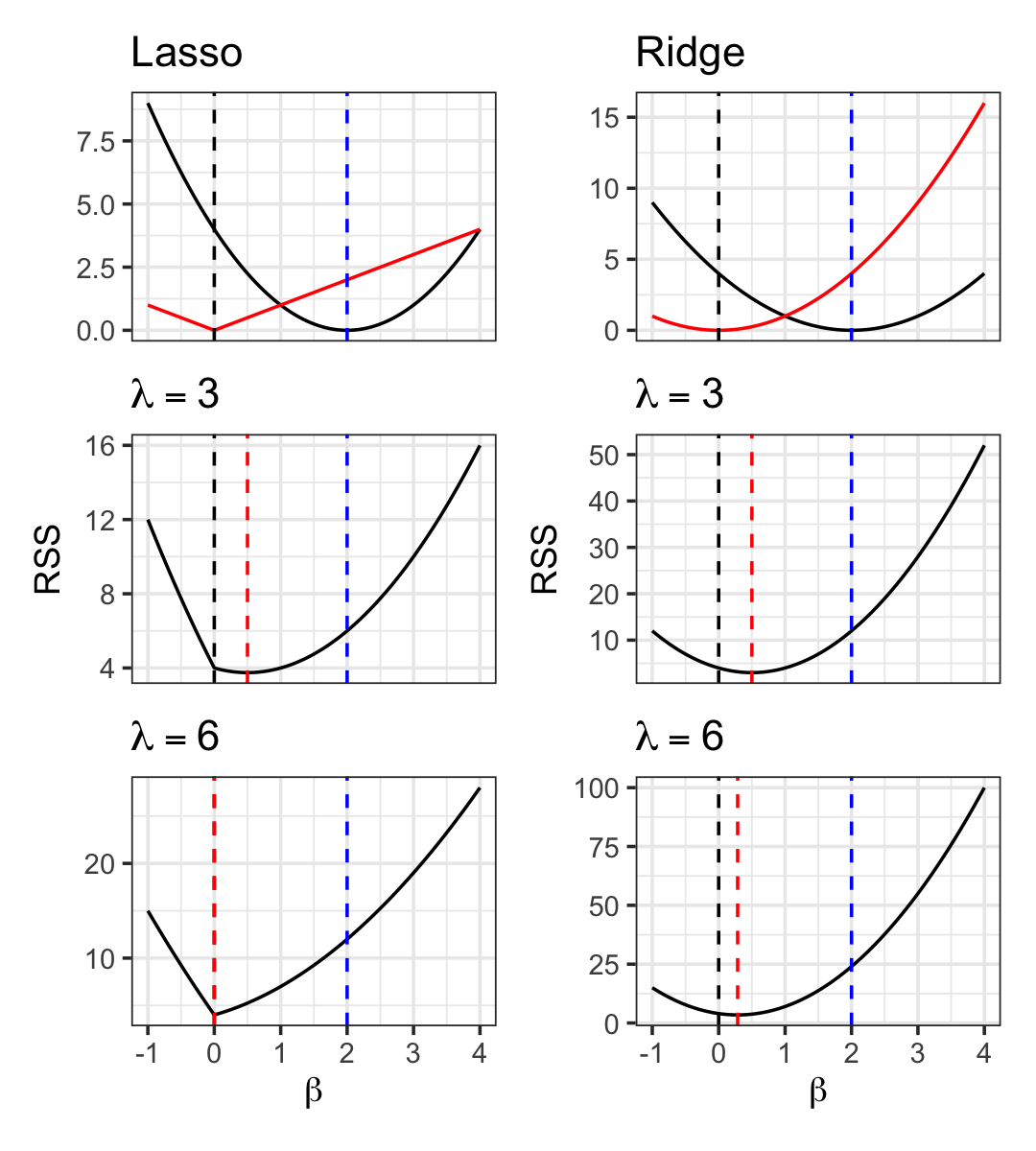
Figure 18.8: Lasso and ridge penalties compared for different values of \(\lambda\). At top, the least-squares loss function is shown in black and the penalty in red. At middle and bottom, the lasso objective (sum of squared loss and penalty) is shown in black for different values of \(\lambda\). The squared-error estimate (blue vertical line) is \(\hat \beta=2\), but increasing \(\lambda\) shrinks the lasso and ridge solutions (red vertical lines) toward 0.

The ridge behavior matches what we saw in Example 18.1, with the solution slowly converging to zero. Lasso, however, does not slowly converge: it jumps to zero between \(\lambda = 3\) and \(\lambda = 6\).

This property is known as sparsity, and there are many real-world populations where we expect the true \(\beta\) to be sparse. For example, a genome-wide association study relates the gene expression levels of thousands of genes to some response (such as a genetic disorder); geneticists often expect only a few of the genes will actually be associated with the response, and the rest have a true coefficient of 0. The goal of the study is to find the few genes with a nonzero relationship.

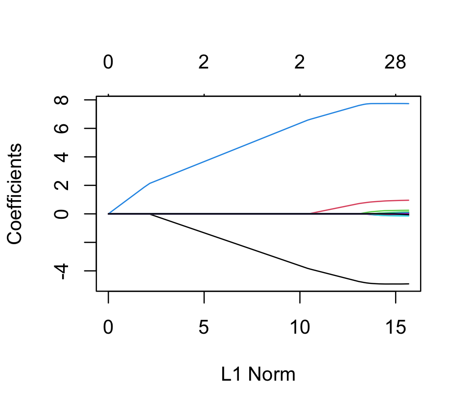
Example 18.5 (Lasso with glmnet) Let’s reuse the sparse population from Example 18.2, but this time use the lasso. It should perform well in a situation like this: many of the predictors have true slopes of exactly 0. We again use glmnet() to do the fit, this time with alpha = 1 to select a pure \(L^1\) penalty.

lasso_fit <- glmnet(x, sparse_samp$y, alpha = 1)

Again, the plot() method for glmnet fits will show the solution path as \(\lambda\) varies, as shown in Figure 18.9.

Figure 18.9: Solution paths for the lasso. Each point on the \(X\) axis represents a lasso fit with a particular penalty parameter. Each line is one estimate \(\hat \beta_j\). On the left, the penalty is the strongest, and only a few parameters have nonzero estimates; as the penalty weakens towards the right, more and more parameters are estimated to be nonzero.

And again, we can use cv.glmnet() to choose the optimal \(\lambda\):

cv_results <- cv.glmnet(x, sparse_samp$y, alpha = 1)
cv_results$lambda.min

[1] 0.09358354

But if we plot the cross-validation results, as in Figure 18.10, we can see that many values of \(\lambda\) have very similar estimated errors—and that the errors of this fit are dramatically lower than the errors in Figure 18.4 for ridge regression.

Figure 18.10: Lasso regression error (estimated by cross-validation) versus the log of the penalty parameter. The error bars indicate estimated standard errors.

This time, most of the truly nonzero coefficients are included among the largest coefficients fit by the model:

coefs <- coef(lasso_fit, s = cv_results$lambda.min)
coefs[order(abs(coefs[, 1]), decreasing = TRUE)[1:15], ]

         x5          x2 (Intercept)          x3         x64         x70 
 7.75316102 -4.93256276  4.06571454  1.05400303 -0.20875636 -0.18865988 
         x1          x4         x55         x43         x77         x49 
 0.13712946  0.12724313  0.11800975 -0.09720581 -0.09105784 -0.07786468 
        x16         x90          x7 
-0.07439692 -0.06965921  0.05386328

If we’re using the lasso in a population we believe is truly sparse, the choice of nonzero coefficients may be of as much interest as the actual values of the nonzero estimates. Identifying the genes associated with a disease, for example, might be just as medically interesting as knowing the actual numerical association. If that is our goal, we want a procedure with model selection consistency.

Definition 18.2 (Model selection consistency) A model selection procedure is a procedure that produces a set of regressors estimated to have nonzero coefficients, \(\{i : \hat \beta \neq 0\}\). Such a procedure is model selection consistent if \[ \Pr(\{i : \hat \beta \neq 0\} = \{i : \beta \neq 0\}) \to 1 \] as \(n \to \infty\).

It can be shown that, under certain conditions, the lasso is model selection consistent (Zhao and Yu 2006). That is, if one knows the “right” value of \(\lambda\), the model selection by lasso is consistent. Typically, of course, we choose \(\lambda\) through cross-validation, and so this property is not guaranteed. (TODO more refs on this?)

There are many variations of the lasso; for instance, the group lasso allows groups of coefficients to be shrunk so that either all of a group is zero or none of them are. This can be used when entering multiple regressors from the same predictor, such as for a factor variable with multiple levels. See Hastie et al. (2015), chapter 4, for more detail.

18.4 The elastic net

We’ve seen two different options for the penalty \(\|\beta\|\) in penalized regression: the Euclidean norm and the Manhattan norm. Each has different properties, and so we might want to choose them in different problems—or we might want to choose a combination of them to solve a combination of problems.

The elastic net uses a combination of ridge and lasso penalties: \[ \hat \beta_\text{elastic} = \argmin_\beta \frac{1}{2n} {\underbrace{\|\Y - \X \beta\|_2^2}_\text{error}} + {\underbrace{\lambda \left(\frac{1 - \alpha}{2} \|\beta\|_2^2 + \alpha \|\beta\|_1\right)}_\text{penalty}}. \] We can see from this form that \(\alpha = 0\) produces ridge regression and \(\alpha = 1\) produces the lasso, but choices in between produce a combination. The combinations trade off the benefits of ridge regression and the lasso: with \(\alpha\) closer to one, more sparsity is induced, but with \(\alpha\) closer to 0, variance from collinearity is reduced more.

18.5 Using penalized models for prediction

We began this chapter by discussing the basic tradeoff of linear models in prediction problems: We want to include many predictors, in case they’re useful, and we want to include many transformed regressors, in case those predictors have a nonlinear relationship with \(Y\). Doing this correctly can yield a good fit, but adding every conceivable predictor with seventh-order polynomials and six-way interactions will likely produce far too much variance. Penalization is a way to eat our cake and have it too: we can add all the regressors, then let the penalization cut the variance.

So suppose we have a few predictors and we wish to build a predictive model for our response. Simply switching from an ordinary linear model to a penalized one, using the same regressors, may or may not help. But we can add regressors to the penalized model without paying the same price as in the un-penalized model. Using cross-validation to choose the penalty parameter \(\lambda\) will automatically adjust the model accordingly: if the new regressors are useless, CV will choose a large penalty; if they’re useful, it will choose a smaller one and allow them to contribute to the model.

Thus there is a temptation to include every possible regressor. I have read a data analysis report from a Ph.D. student who was asked to predict a response from numerous predictors—in fact, a very similar problem to the case study in Chapter 26—and decided to consider 23 predictors. To ensure the model was flexible enough, those 23 predictors were combined to produce 3,030 additional interaction terms. (Actually there were 8,680, but many were always zero, so they were removed.) Then the lasso was used to reduce this down to just 14 regressors.

This approach reminds me of the story from the Albigensian Crusade: while massacring the Cathars in 1209, the Crusade’s leader was asked how to tell apart Cathars and Catholics. He (allegedly) replied “Kill them. The Lord knows those that are His.” (Caedite eos. Novit enim Dominus qui sunt eius.) Thus this approach of choosing regressors with penalized regression might be described as “Include them all. The penalty knows those that are real.”

Whether or not you take this approach to the extreme of considering 3,030 interaction terms, it is reasonable to use penalized models with additional regressors to allow more flexible fits. One must only remember to cross-validate the fitting procedure in the correct order (Section 17.3.5) so error estimates correctly account for the uncertainty in choosing the correct penalty \(\lambda\).

18.6 Inference

Inference for the parameters of any penalized regression model is complicated by several factors:

The estimator is no longer a maximum likelihood estimator, so we can’t fall back on maximum likelihood theory. The Fisher information will not give us \(\var(\hat \beta)\) (Theorem 12.1), and the likelihood ratio test (Theorem 11.2) will not be valid.
The fit depends on our choice of penalty parameter \(\lambda\), which we usually choose based on the data, creating a post-selection inference problem (Section 11.5).
In lasso and the elastic net, the sampling distribution of each parameter \(\hat \beta_j\) includes a point mass at 0. Thus it is not a nice, symmetric, approximately normal distribution, so Wald tests and confidence intervals won’t work even if we can derive the standard error of the estimates.

Typically penalized models are used in prediction problems where inference is not necessary, so these issues are not important. Model reporting focuses on prediction error estimates from cross-validation, rather than on significance tests or confidence intervals.

If inference is desired, TODO

Exercises

Exercise 18.1 (Ridge regression estimator) Derive the ridge regression estimator, \[ \hat \beta_\text{ridge} = (\X\T\X + 2n \lambda I)^{-1} \X\T\Y, \] from the definition of the ridge objective function in Section 18.2.

Exercise 18.2 (Choosing the penalty parameter) Suppose you observe \(n\) samples from a population with \(Y \in \R\) and \(X \in \R^p\). You decide a linear model would be appropriate, and that the lasso would be useful because you suspect the problem is sparse. You decide to set the penalty parameter \(\lambda\) and estimate the error of the final model through the following procedure:

Split the data into a training set and test set of equal sizes.
Fit the model to the training set using a certain \(\lambda\). Evaluate its error on the test set.
Repeat step 2 with many values of \(\lambda\), using the same training and test sets each time.
Pick the \(\lambda\) that gives the best test error. Report its test error as our estimate of the generalization error of the fitted model.

Will this test-set error be an accurate estimate of the model’s generalization error on new data? If yes, describe why; if not, suggest an alternate procedure to estimate the generalization error accurately.

Hint: As a simple example, consider what would happen if all values of \(\lambda\) had equal generalization error. Recall that test error calculated from real data is a random quantity.

Exercise 18.3 (Penalized regression with correlated predictors) Consider a sparse population where only two predictors are associated with the response, but they are highly correlated with each other:

library(regressinator)
library(mvtnorm)

# unit variance
sigma <- diag(5)

# but X1 and X2 are correlated
sigma[1, 2] <- 0.75
sigma[2, 1] <- 0.75

sparse_corr_pop <- population(
  x = predictor(rmvnorm,
                mean = rep(0, 5),
                sigma = sigma),
  y = response(
    7 + x1 + x2,
    error_scale = 1
  )
)

Obtain 1000 draws from the sampling distribution of \(\hat \beta_1\) and \(\hat \beta_2\), estimated using ordinary least squares, on samples of size \(n = 50\) from this population. Fit each model including all predictors.

Make a plot of the joint distribution of \(\hat \beta_1\) and \(\hat \beta_2\), such as a scatterplot or a 2D density estimate. (See, for instance, ggplot2’s geom_density_2d().)
Repeat this procedure but with ridge regression, with \(\lambda = 1\). In glmnet(), set standardize = FALSE so it does not automatically standardize the regressors—this makes the penalty comparable between simulated datasets.

Make a similar plot of the joint distribution. Use the same axis ranges to ensure your plots are comparable.

Note: Unfortunately, the regressinator’s sampling_distribution() does not work with models fit by glmnet(). But you can use replicate() to do this easily, by filling in the missing pieces here:
```
replicate(1000, {
  new_samp <- sparse_corr_pop |>
    sample_x(n = 50) |>
    sample_y()

  x <- # TODO get X matrix
  y <- # TODO get Y matrix
  fit <- glmnet(TODO, alpha = 0, lambda = TODO,
                standardize = FALSE)

  coefs <- coef(fit)

  coefs[2:3] # 1 is the intercept
})
```
This will produce a \(2 \times 1000\) matrix containing each simulation’s values of \(\hat \beta_1\) and \(\hat \beta_2\).
Finally, repeat the procedure with lasso and \(\lambda = 1\). (The true parameter vector is \(\beta = (1, 1, 0, 0, 0)\T\), so \(\|\beta\|_2^2 = 2\) and \(\|\beta\|_1 = 2\). The penalties are hence comparable as long as you keep standardize = FALSE.) Again, make a plot of the joint distribution, using the same axis scales as before.
Based on your three plots, comment on the bias of lasso and ridge regression. Are they unbiased? How biased are they?
Based on your three plots, comment on the shape of the sampling distributions. The least squares distribution should show a noticeable correlation between \(\hat \beta_1\) and \(\hat \beta_2\), which is what we expect when predictors are collinear; what about lasso and ridge? Explain why the nature of their penalty functions explains their differing behavior with collinear predictors.

This problem illustrates why ridge regression is popular in settings with highly collinear predictors, and why it can produce estimates with low variance even in those settings. When a problem is both sparse and has collinear predictors, this problem illustrates why the elastic net can be useful.

Exercise 18.4 (Ridge regression and collinearity) We can also see the appeal of ridge regression problems with collinearity by appealing to the math of Section 9.5, where we saw that collinearity is connected to the eigenvalues of \(\X\T\X\).

TODO Hastie et al. (2009) pages 64-68

Exercise 18.5 (Gene expression and autism) (This problem is based on the Data Analysis Exam given to Ph.D. students in Statistics in 2013.)

The occurrence of autism is believed to be related to gene expression, at least in part. Gene expression refers to the process by which genes are used to synthesize proteins that serve functions in the cell; gene expression levels indicate how much each gene is being expressed. Gene expression is regulated by various genetic and epigenetic mechanisms: people with the same genes may express them in different amounts. If the gene regulation mechanism operates differently, it may affect traits like autism by altering which proteins and products are produced in the brain.

The file genedat-exam.csv on Canvas contains gene expression data from 19 people with autism and 17 people without. This is measured using microarrays, which can measure the expression of many genes at the same time; in this dataset, we have selected 125 genes, but there were nearly 20,000 measured in the original study. Some of the people had expression levels measured in both their frontal cortex and temporal cortex, and these appear as separate rows in the data, making 58 rows in total. We have the following columns:

CaseID: ID number for each person
Cortexarea: frontal or temporal cortex
Disease: autism or control
RIN: RNA integrity number, a measure of the quality of the microarray measurement. Above 7 is good quality, and above 5.5 is considered acceptable.
Age: Age of the person measured
Sex: Sex of the person measured

There then follow 125 columns giving gene expression levels for different genes.

Choose the appropriate type of GLM to use for this data. Why can you not fit it directly with maximum likelihood and no penalty?
Build lasso and ridge GLMs to predict autism status using the gene expression data. Use cross-validation to select the tuning parameters.
Write a function that uses predict() to predict autism status for each observation in a data frame, by predicting autism if the predicted probability is 0.5 or greater.
Using the tuning parameters you selected in part 2, use cross-validation to evaluate the accuracy of lasso and ridge. Which performs best?
Describe a more appropriate way to design the analysis so your cross-validated comparison of the two models is unbiased and gives valid error estimates. (Recall Section 17.3.5 on selecting tuning parameters in cross-validation.)