17 Prediction Goals and Prediction Errors

So far in this course, we have considered problems where our goal is to infer features of the true relationship \(\E[Y \mid X = x]\). We might want to test if a particular predictor is relevant, determine if a relationship is positive, or estimate a particular parameter. This goal requires fitting an appropriate model, using diagnostics to determine if it fits well, and then using inference procedures appropriate for our question of interest.

But often our goal is more straightforward. We imagine there is a true population joint distribution, so that \((X, Y) \sim F\), where \(F\) is some unknown distribution. We have a set of training observations \((x_1, y_1), (x_2, y_2), \dots, (x_n, y_n)\). If we obtain a new draw \(X^*\) from \(F\), how do we best predict the matching \(Y^*\)?

Many real problems are like this. We may not care what the exact shape of the relationship is or want to learn about it—we just want to make predictions. A spam filter just needs to make the best possible classifications; a social media recommendation algorithm just needs to predict which content you’ll like; a high-frequency trading algorithm just needs to predict changes in stock prices.¹ It may be interesting to do inference and learn how features are associated with the response, but it is not necessary.

Prediction raises two simple questions:

How do we define the “best” predictions?
How do we measure how well a model predicts, so we can pick the best one?

17.1 Risk and loss

First we can define the goodness of a prediction. Suppose we have a vector of predictors \(X \in \R^p\) and a response variable \(Y\) we want to predict, drawn from a population distribution \((X, Y) \sim F\). We draw a training set \(\trainset = \{(x_1, y_1), \dots, (x_n, y_n)\}\). We use the training set to estimate a function \(\hat f(X)\), and we predict \(\hat Y = \hat f(X)\).

Definition 17.1 (Loss function) A loss function is a bivariate function \(L(Y, \hat f(X))\) whose value is interpreted as the “loss” of \(\hat f(X)\) for predicting \(Y\). A larger loss represents a worse prediction.

Some common loss functions include:

Squared error: \[ L\left(Y, \hat f(X)\right) = \left(Y - \hat f(X)\right)^2 \]
Absolute error: \[ L\left(Y, \hat f(X)\right) = \left|Y - \hat f(X)\right| \]
Cross-entropy loss, when \(Y \in \{0, 1\}\) and \(\hat f(X) = \widehat{\Pr}(Y = 1 \mid X)\): \[ L\left(Y, \hat f(X)\right) = Y \log(\hat f(X)) + (1 - Y) \log(1 - \hat f(X)) \]
Deviance, when \(\ell(\beta)\) is the log-likelihood given the observed data and the model \(\hat f(X)\): \[ L(Y, \hat f(X)) = - 2 \ell(\hat \beta). \]

We choose loss functions depending on the response variable and our prediction goals; for continuous response variables, squared error loss is the popular default, but we might choose absolute error to prevent outliers from being influential, or choose an asymmetric loss if overestimation and underestimation have different costs. For binary outcomes, the cross-entropy loss is the same as the log-likelihood used in logistic regression (Section 12.2).

Once we have selected a loss function, we can define the generalization error.

Definition 17.2 (Generalization error) The generalization error, test error, or prediction risk of a model \(\hat f(X)\) trained on a training set \(\trainset\), relative to a loss function \(L(Y, \hat f(X))\), is \[ R_{\trainset} = \E[L(Y, \hat f(X)) \mid \trainset], \] where the expectation is over new draws of \((X, Y)\) from their population joint distribution.

The generalization error is exactly what we want to know: With this model, fit to the training data we have, how much error (loss) can we expect when making predictions on new data? If we have several candidate models, we could estimate the generalization error for each and choose the model with the best results.

However, we will find the generalization error to be quite hard to estimate. Instead, we’ll estimate the expected prediction error.

Definition 17.3 (Expected generalization error) The expected generalization error, expected prediction error or expected test error of a model \(\hat f(X)\), relative to a loss function \(L(Y, \hat f(X))\), is \[ R = \E[L(Y, \hat f(X)] = \E[R_{\trainset}], \] where the outer expectation is over the training set \(\trainset\) as well as the test point \((X, Y) \sim F\).

Definition 17.3 is an abuse of notation and hides its meaning behind a deceptively simple definition. The expected generalization error \(R\) is a property of the estimation procedure for \(\hat f(X)\) and the size \(n\) of the training set: If we draw any training set \((x_1, y_1), \dots, (x_n, y_n)\) from \(F\), fit the model \(\hat f(X)\), and then draw any new observation \((X^*, Y^*) \sim F\), what is the expected loss \(L(Y^*, \hat f(X^*))\)?

This is simultaneously more revealing—it tells us which model or estimator is best-suited to the population \(F\)—and less useful, because it doesn’t tell us which model is best given the particular training set \(\trainset\) we have. A model may have a poor generalization error because of an unlucky training sample, even if it is well-suited to the population relationship and has a great expected generalization error.

Also, notice the proliferation of names (test error, prediction risk, expected test error, and so on). These names are used inconsistently by different authors: sometimes “test error” refers to the expected generalization error; sometimes it refers to the error on a specific test set rather than an expectation; sometimes no distinction is made between the two kinds of error.

Finally, we can define the error on our training sample alone, without appeal to any populations and expectations.

Definition 17.4 (Training error) The training error of a model \(\hat f(X)\) trained on a training set \(\trainset = \{(x_1, y_1), \dots, (x_n, y_n)\}\), relative to a loss function \(L(Y, \hat f(X))\), is \[ R_\text{train} = \frac{1}{n} \sum_{i=1}^n L(y_i, \hat f(x_i)). \]

The training error is easy to calculate whenever we have fit a model to training data. However, as we will see in Section 17.5, the training error is a poor estimator of the generalization error.

17.2 Metrics for classification

In classification problems, where \(Y\) only takes discrete values, measuring loss gets more interesting. Some classifiers, like logistic regression, produce predicted probability values, and we could use \(\hat f(x) = \widehat{\Pr}(Y = 1 \mid X = x)\) in a standard loss function like squared error. But other classifiers may only produce a predicted \(\hat Y\), not a probability. And the loss doesn’t tell the whole story; we may want to break down specific types of errors. Let’s consider the options.

17.2.1 Breaking down the confusion matrix

For classifiers, we can create a confusion matrix using the training data or a test set. The confusion matrix is a contingency table counting the number of observations with each response value, cross-classified by the model’s predicted response value. A typical confusion matrix for binary classification is shown in Table 17.1.

Table 17.1: A typical confusion matrix for binary classification. Each cell would contains counts of observations, based on \(Y\) and \(\hat Y\).

Actual	\(\hat Y = 1\)	\(\hat Y = 0\)	Total
\(Y = 1\)	True positive (TP)	False negative (FN)	Positives (P)
\(Y = 0\)	False positive (FP)	True negative (TN)	Negatives (N)
Total			Population (\(n\))

In binary classification, we speak generically of \(Y = 1\) being a “positive” and \(Y = 0\) being a negative. (The naming comes from medical testing, where you can “test positive” or “test negative” for a disease.) The confusion matrix lets us count true positives and negatives, where \(\hat Y = Y\), and false positives and negatives, where \(\hat Y \neq Y\). Using these counts, we can derive lots of summaries.

Definition 17.5 (Binary classification metrics) In a binary classification task, the confusion matrix (Table 17.1) can be summarized in many ways. First, consider dividing by the row totals (the actual counts):

Actual	\(\hat Y = 1\)	\(\hat Y = 0\)
\(Y = 1\)	True positive rate, recall, sensitivity: \(\text{TPR} = \text{TP} / \text{P}\)	False negative rate: \(\text{FNR} = \text{FN} / \text{P}\)
\(Y = 0\)	False positive rate: \(\text{FPR} = \text{FP} / \text{N}\)	True negative rate, specificity: \(\text{TNR} = \text{TN} / \text{N}\)

Next, divide by the column totals:

Actual	\(\hat Y = 1\)	\(\hat Y = 0\)
\(Y = 1\)	Positive predictive value, precision: \(\text{PPV} = \text{TP} / (\text{TP} + \text{FP})\)	False omission rate: \(\text{FOR} = \text{FN} / (\text{FN} + \text{TN})\)
\(Y = 0\)	False discovery rate: \(\text{FDR} = \text{FP} / (\text{TP} + \text{FP})\)	Negative predictive value: \(\text{NPV} = \text{TN} / (\text{FN} + \text{TN})\)

We can also define the accuracy, \((\text{TP} + \text{TN})/n\), the fraction of correct predictions.

These statistics are often expressed as percentages.

Accuracy is, of course, the most popular summary. But accuracy on its own is not sufficient to describe the behavior of a classifier.

Example 17.1 (Accuracy in a medical test) Suppose you are assigned to build a classifier that takes a patient’s blood test results (\(X\)) and predicts whether they have cancer (\(Y = 1\)). Observing the true \(Y\) requires invasive and expensive biopsies, so you’d like a highly accurate classifier using the much cheaper blood test results.

In the population, only 1 in 100,000 people have this cancer. Consequently, the simple classifier \(\hat f(x) = 0\) has 99.999% accuracy when applied to a random sample of people. However, proposing this classifier will get you kicked out of the American Association for Cancer Research annual meeting.

This example illustrates that accuracy is never useful unless also presented with the base rates of each class. Alternately, if presenting a table of accuracies of various models, include a baseline model that always predicts the majority class.

The example also suggests why the other confusion matrix summaries are useful. The dumb classifier has great accuracy, but its true positive rate is 0! That is, the metrics break down the 0.001% of cases that are misclassified so we can see exactly what kind of errors are being made, and the true positive rate makes it clear that we are making errors by never detecting positive cases.

Similarly, the positive predictive value is useful: If the classifier reports \(\hat Y = 1\), what is the probability that \(Y = 1\)? If the test says I have cancer, what is the probability I actually do? For a cancer screening test, we want to balance positive predictive value and sensitivity; it is bad to miss cancer cases (low sensitivity), but it is also bad to waste resources by reporting many false positives that must be investigated (low positive predictive value). Choosing the right classifier might require balancing these properties with the cost of each type of error.

Naturally, there are many statistics that try to compute a one-number summary that is more useful than the accuracy, balancing each kind of error in one figure. The most popular is the \(F_1\) score.

Definition 17.6 (\(F_1\) score) For a binary classifier, the \(F_1\) score is the harmonic mean of the true positive rate (recall) and the positive predictive value (precision): \[ F_1 = \frac{2}{\text{TPR}^{-1} + \text{PPV}^{-1}} = \frac{2 \text{TP}}{2\text{TP} + \text{FP} + \text{FN}}. \] The \(F_1\) score is bounded between 0 and 1; a perfect model scores 1 and a model with 0 TPR or PPV scores 0.

You will find the \(F_1\) score widely used as a general-purpose summary of classifier performance, particularly for things like prediction competitions.

Example 17.2 (Performance of the Pima diabetes classifier) In Example 12.5 we introduced a model for predicting the presence of diabetes among Pima women. The dataset comes in two parts, a training set and a test set, so we can fig the model to the training set and evaluate it on the test set. We begin by fitting the model on the training data.

library(MASS)

Pima.tr$pregnancy <- factor(
  ifelse(Pima.tr$npreg > 0, "Yes", "No")
)

pima_fit <- glm(type ~ pregnancy + bp, data = Pima.tr,
                family = binomial())

We can obtain the predicted probabilities on the test data, and also threshold these at 0.5 to give the predicted diabetes status. To do so, we need to introduce the pregnancy variable in the test data as well:

Pima.te$pregnancy <- factor(
  ifelse(Pima.te$npreg > 0, "Yes", "No")
)
pima_preds <- predict(pima_fit, newdata = Pima.te, type = "response")
predicted_status <- ifelse(pima_preds >= 0.5, "Yes", "No")

A confusion matrix is easy to produce with R’s xtabs() function, if we put the predictions and true values in a data frame first.

compare_df <- data.frame(
  predicted = predicted_status,
  true = Pima.te$type
)

contingency <- xtabs(~ predicted + true, data = compare_df)
contingency

         true
predicted  No Yes
      No  204  99
      Yes  19  10

From this we can compute any measures we want. TODO

17.2.2 Metrics with varying thresholds

For many classifiers, we don’t simply obtain \(\hat Y \in \{0, 1\}\). We may get a score that varies over an interval, and use a cutoff to assign \(\hat Y\). For example, in logistic regression we estimate \(\widehat{\Pr}(Y = 1 \mid X = x) \in [0, 1]\), and typically set a threshold of 0.5 for assigning \(\hat Y\) to be 0 or 1. Many other classifiers, like random forests or neural networks, can also give scores or estimated probabilities that we threshold.

But nobody says we have to use 0.5, or that 0.5 is guaranteed to give the best tradeoff between types of errors. We can, in principle, compute a confusion matrix for every possible threshold, then choose the best threshold. We could also select the classifier that performs best across the entire range of thresholds, rather than the one that does best at one specific cutoff. This leads us to the idea of plotting the performance across the range of threshold values. Because different models may have different ranges of scores, instead of plotting against the threshold we plot two error metrics against each other.

Definition 17.7 (ROC curve) The receiver operating characteristic (ROC) curve for a binary classification model is a plot of the false positive rate (on the \(X\) axis) against the true positive rate (on the \(Y\) axis) as the threshold is varied across its range.

The area under the curve (AUC) is the integral of this curve. Because the true and false positive rates are bounded between 0 and 1, the AUC is bounded between 0 and 1 as well.

You might wonder about the name—a lot of classification error names come from medical testing, so what is the “receiver” in ROC? It’s a radar receiver, since the technique comes from tests of radar’s ability to detect aircraft during World War II.

A plotted ROC curve implicitly contains a comparison to a baseline model.

Theorem 17.1 (ROC of a random classifier) Consider a random classifier that predicts the positive class with probability \(p\), regardless of covariates. If we treat \(p\) as the prediction threshold, this classifier will have a perfectly diagonal ROC curve.

Proof. The proof is trivial: the false positive rate is \(p\) because that fraction of negative cases are predicted positive, and the true positive rate is \(p\) because that fraction of positive cases are predicted positive.

Consequently, the baseline model should have an AUC of 0.5. Any classifier with a lower AUC is performing worse than classifying randomly.

Example 17.3 (Pima ROC curve) Continuing from Example 17.2, we can produce an ROC curve for our logistic regression model. There are many packages to compute ROC curves, but here we will use ROCR, which can plot many different performance measures.

library(ROCR)

pred <- prediction(pima_preds, Pima.te$type)
plot(performance(pred, measure = "tpr", x.measure = "fpr"))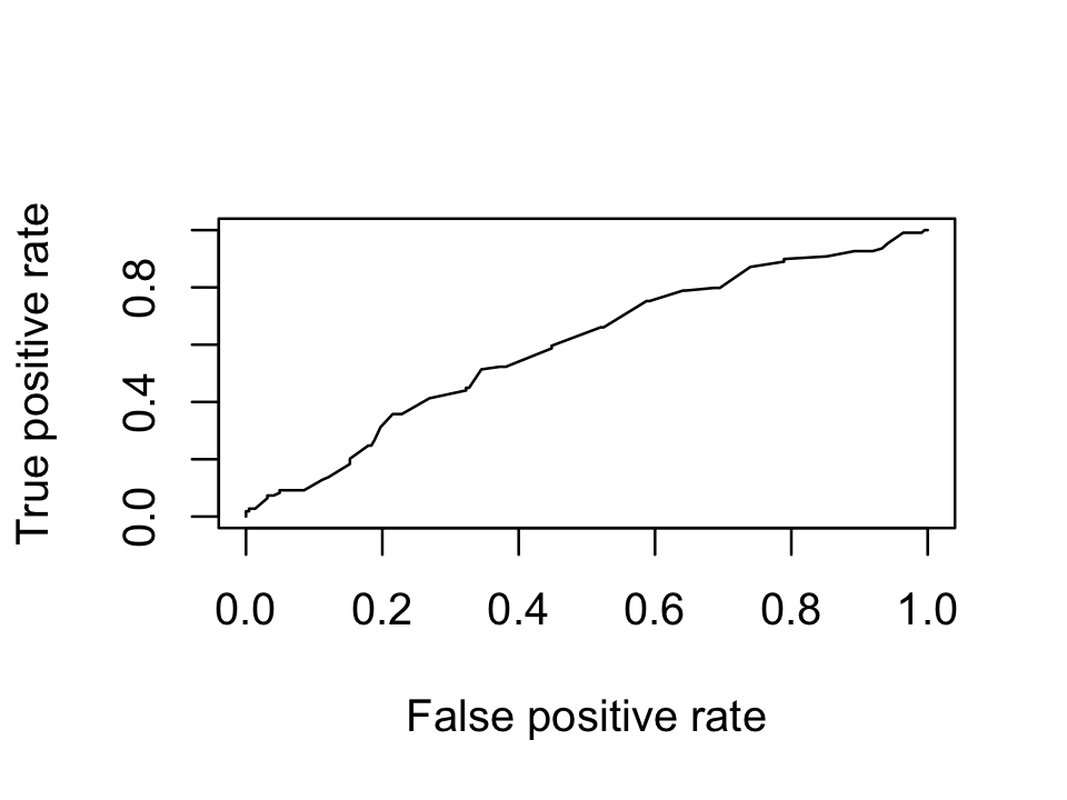

Figure 17.1: ROC curve for predictions of diabetes status in Pima women.

The AUC is not very good:

performance(pred, measure = "auc")@y.values

[[1]]
[1] 0.5963508

Often you will see multiple classifiers compared by plotting their ROC curves together on one plot.

TODO proper scoring

17.3 Bias, variance, and the bias-variance decomposition

Hastie, Tibshirani, and Friedman (2009), section 7.3

The squared error loss has useful properties that will help us build intuition for the trade-offs between different prediction methods. One of these properties is so useful that it gets its own name: the bias-variance decomposition.

Consider the usual regression setting where \(Y \in \R\) and \(Y = \E[Y \mid X = x] + e\), where \(e\) is mean-0 noise. Intuitively, we can see that the prediction error can come from several sources:

Irreducible error: Even if we estimate \(\E[Y \mid X = x]\) perfectly, if \(\var(e) > 0\), we cannot predict \(Y\) perfectly. The error due to \(e\) is the irreducible error.
Bias: Our estimate of \(\E[Y \mid X = x]\) may be biased. Perhaps we are using a linear model when the relationship is not linear, or perhaps we are using a penalized model (Chapter 19), so our estimated regression has systematic error.
Variance: Even if our estimator is unbiased, there is sampling variation: we will obtain a different model fit for every training set.

Each of these errors can be rigorously defined, and the squared-error prediction risk can be written in terms of them. It’s easiest to start by doing so for point estimation before moving to regression.

17.3.1 In point estimation

Consider a standard point estimation problem, we obtain a sample \[ Y_1, \dots, Y_n \sim F(\theta), \] where \(F\) is some parametric distribution with unknown parameter \(\theta\). We’d like to estimate \(\theta\), so we define an estimator \(\hat \theta_n\), which is a function of \(Y_1, \dots, Y_n\).

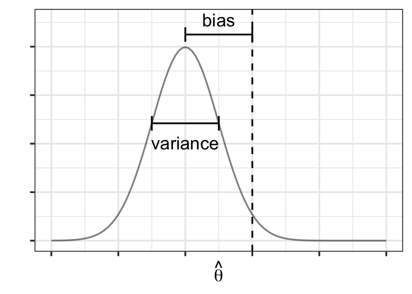
We define the bias of \(\hat \theta_n\) as \(\bias(\hat \theta_n) = \E[\hat \theta_n] - \theta\), where the expectation averages over random samples from \(F\). The variance of \(\hat \theta_n\) is again defined across repeated samples: \(\var(\hat \theta_n) = \E\left[(\hat \theta_n - \E[\hat \theta_n])^2\right]\). The bias and variance of \(\hat \theta\)’s sampling distribution are illustrated in Figure 17.2.

Figure 17.2: Sampling distribution of an estimator \(\hat \theta\). The estimator is biased relative to the true value \(\theta\) (vertical dashed line), and has sampling variance.

The total mean squared error of the estimator can be written in terms of its bias and variance.

Theorem 17.2 (Bias-variance decomposition for point estimates) The mean-squared error of a point estimator \(\hat \theta_n\) for a parameter \(\theta\), defined to be \[ \MSE(\hat \theta_n) = \E\left[(\hat \theta_n - \theta)^2\right], \] can be written as \[ \MSE(\hat \theta_n) = \var(\hat \theta_n) + \bias(\hat \theta_n)^2. \]

Proof. We expand out the square: \[\begin{align*} \MSE(\hat \theta_n) &= \E\left[ \left( (\hat \theta_n - \E[\hat \theta_n]) + (\E[\hat \theta_n] - \theta)\right)^2 \right]\\ &= \E\left[ (\hat \theta_n - \E[\hat \theta_n])^2 + (\E[\hat \theta_n] - \theta)^2 + 2 (\hat \theta_n - \E[\hat \theta_n]) (\E[\hat \theta_n] - \theta)\right]\\ &= \var(\hat \theta_n) + \bias(\hat \theta_n)^2 + 0, \end{align*}\] as the expectation of the third term is 0.

This decomposition allows us to better understand the tradeoffs between estimators. For instance, it’s intuitive to always use unbiased estimators, because “unbiased” sounds like a good property; but do unbiased estimators always have the lowest error? No!

Example 17.4 (Estimating the mean) Suppose we observe \(Y \sim \normal(\mu, \sigma^2)\) and we want to estimate \(\mu\).

The minimum variance unbiased estimator of \(\mu\) is \(Y\). But consider instead the estimator \(\hat \mu = \alpha Y\), where \(0 \leq \alpha \leq 1\). We have \[\begin{align*} \E[\hat \mu] - \mu &= \E[\alpha Y] - \mu\\ &= \alpha \mu - \mu\\ &= (\alpha - 1) \mu, \end{align*}\] so the estimator is biased if \(\alpha \neq 1\). For variance, we have \[\begin{align*} \var(\hat \mu) &= \var(\alpha Y)\\ &= \alpha^2 \sigma^2. \end{align*}\] Adding the squared bias and variance, we have \[ \MSE(\hat \mu) = (1 - \alpha)^2 \mu^2 + \sigma^2 \alpha^2. \] As \(\alpha \to 1\), the bias goes to 0 and the variance increases. As \(\alpha \to 0\), the bias increases and the variance decreases. The MSE is minimized at \[ \alpha = \frac{\mu^2}{\sigma^2 + \mu^2} < 1, \] so surprisingly enough, the lowest-MSE estimator is also biased toward 0.

We can apply a similar decomposition to regression, and it will lead to similar realizations: in Chapter 19, we’ll consider deliberately biasing models to decrease their error.

17.3.2 In regression

To apply the bias-variance decomposition to regression, let’s simplify the problem. Regression involves estimating a function, not a point value, but if we condition on a specific value \(X = x\), then estimating \(\E[Y \mid X = x]\) is a point estimation problem. So let’s adapt the expected generalization error (Definition 17.3) to point estimation.

Definition 17.8 (Conditional generalization error) The generalization error conditional on \(X = x\) is \[ R(x) = \E\left[L(Y, \hat f(X)) \mid X = x\right], \] where the expectation is over both training sets \(\trainset\) and response values \(Y\) drawn from the conditional distribution \(F_{Y \mid X = x}(Y)\).

We can obtain the expected generalization error by marginalizing the conditional generalization error: \[ R = \E[R(x)] = \int R(x) f_X(x) \dif x, \] where \(f_X(x)\) is the marginal density of \(X\).

Now we’re ready to prove the bias-variance decomposition for regression.

Theorem 17.3 (Bias-variance tradeoff for regression) In a regression problem where \(Y = f(X) + e\), the conditional generalization error for the squared-error loss can be decomposed as \[ R(x) = \var(\hat f(x) \mid X = x) + \bias(\hat f(x) \mid X = x)^2 + \var(e \mid X = x). \]

Proof. By definition, \[\begin{align*} R(x) ={}& \E[(Y - \hat f(X))^2 \mid X = x] \\ ={}& \E\left[ (Y - f(X) + f(X) - \hat f(X))^2 \mid X = x \right]\\ ={}& \E\left[ (Y - f(X))^2 \mid X = x \right] + \E\left[ (f(X) - \hat f(X))^2 \mid X = x \right] \\ &{}+ 2 \E\left[(Y - f(X))(f(X) - \hat f(X)) \mid X = x\right]\\ ={}& \var(e \mid X = x) + \E\left[(\hat f(x) - f(x))^2\right] + 0. \end{align*}\] The last term is zero because here, \(Y\) is a new observation independent of the training set \(\trainset\) and hence independent of \(\hat f(x)\).

The second term is the MSE of \(\hat f(x)\) for estimating \(f(x)\). Following Theorem 17.2, it can be broken into bias and variance.

The bias-variance tradeoff implies that the best generalization error may be achieved by a model that compromises between bias and variance—by a model that is biased. We can deliberately introduce bias if it reduces the variance of the estimator.

Exercise 17.1 (The bias-variance tradeoff) Let’s explore the bias and variance in a specific concrete example, and explore how we might tune a model to achieve the right balance.

We’ve previously used the Doppler function, for instance when discussing polynomials (Figure 10.3) and fitting smoothing splines (Example 14.1). Here’s a population where the relationship between \(X\) and \(Y\) is given by the Doppler function:

library(regressinator)

doppler <- function(x) {
  sqrt(x * (1 - x)) * sin(2.1 * pi / (x + 0.05))
}
doppler_pop <- population(
  x = predictor(runif, min = 0.1, max = 1),
  y = response(
    doppler(x),
    error_scale = 0.2
  )
)

Let’s consider taking a sample of \(n = 50\) observations and fitting a smoothing spline. We’ll set the effective degrees of freedom for our spline, which is equivalent to setting the penalty parameter \(\lambda\), and try different values to see their bias, variance, and total error. This can be done by using smooth.spline() with the df argument; see Example 14.1 to see how smooth.spline() is used.

Write a loop to try different values of the effective degrees of freedom, from 5 to 24. For each edf,

Sample \(n = 50\) observations from doppler_pop.
Fit a smoothing spline with the chosen edf.
Use that smoothing spline to obtain a prediction at \(x_0 = 0.2\).
Store the prediction in a data frame, along with the edf used to obtain it.
Repeat steps 1-4 500 times.

You should now have a data frame with \(20 \times 500\) rows, for 20 edfs and 500 simulations each.

For each edf, estimate the squared bias \(\E[\hat f(x_0) - f(x_0)]^2\); you can use doppler(0.2) to get \(f(x_0)\). Also, for each edf, estimate the variance \(\E\left[\left(\hat f(x_0) - \E[\hat f(x_0)]\right)^2\right]\).

Make a plot of squared bias versus edf and a plot of variance versus edf.

TODO mention Belkin et al. (2019), Hastie et al. (2022)

17.4 The curse of dimensionality

17.5 Optimism of the training error

Hastie, Tibshirani, and Friedman (2009), section 7.4

All this discussion of prediction error leads to an obvious question: How do we estimate it? If I have several different predictive models and want to know which generalizes the best, how do I do that?

The obvious answer would be to use the training error (Definition 17.4), as it can be calculated directly from the training data. However, it should be obvious that this is not always wise. In linear regression, for instance, we can always obtain a perfect fit (zero training error) by having as many regressors as training observations, even if the true population relationships are nonlinear. Evidently the training error can be optimistic, in that it is lower than the generalization error.

We can quantify this optimism. It is easiest to do so by comparing the training error to the in-sample prediction error.

Definition 17.9 (In-sample prediction error) The in-sample prediction error of a model \(\hat f(X)\) trained on a training set \(\trainset\), relative to a loss function \(L(Y, \hat f(X))\), is \[ R_\text{in} = \frac{1}{n} \sum_{i=1}^n \E[L(Y_i^*, \hat f(x_i)) \mid \trainset], \] where the expectation is over new draws \(Y_i^*\) from the conditional distribution given \(X = x_i\).

The in-sample prediction error eliminates one source of variation: we make our predictions at the same \(X\) values, but obtain new response values at those points. There is no error introduced by extrapolating to new \(X\) values. This is unsuitable for typical prediction problems (where each observation to predict is a new draw from the population), but matches the standard linear regression setting where \(X\) is considered fixed.

We can now calculate the optimism of the training error relative to the in-sample prediction error.

Theorem 17.4 (Optimism of the training error) Given a model \(\hat f(X)\) trained on a training set \(\trainset\), the optimism of the training error is \[ \text{opt} = R_\text{in} - R_\text{train}. \] The average optimism \(\omega\) averages over training sets \(\trainset\), and one can show that for squared-error loss, \[\begin{align*} \omega &= \E[\text{opt}] \\ &= \frac{2}{n} \sum_{i=1}^n \cov(\hat f(x_i), Y_i)\\ &= \frac{2 \sigma^2}{n} \edf(\hat f), \end{align*}\] where the effective degrees of freedom \(\edf(\hat f)\) is defined in Definition 14.2.

Proof. See Exercise 17.2.

In short, a more flexible model (one with more effective degrees of freedom) will have greater optimism: on average, across all training sets, its training error will be substantially less than the true in-sample prediction error. On average, then, picking the model with the best training error amounts to picking the most flexible model, not the model with the best prediction error.

We can generalize this result from squared-error loss to deviance, when we measure performance using the log-likelihood.

Theorem 17.5 (Optimism of the log-likelihood) Given a model with parameters \(\beta \in \R^p\) with log-likelihood function \(\ell(\beta)\), consider \(\E[\ell^*(\beta)]\), the expected value of the log-likelihood when evaluated on a new independent draw from the population. As \(n \to \infty\), the optimism of the training log-likelihood is \[ \E[\ell(\hat \beta)] - n \E[\ell^*(\hat \beta)] \approx p. \]

Proof. See Pawitan (2001), section 13.6.

This implies that optimism is a problem for any likelihood-based model, in that it will fit better to the training data than to new, independent test data. In the next chapter, we’ll introduce alternate ways to estimate the prediction error that avoid this bias.

Exercises

Exercise 17.2 (Optimism) Prove Theorem 17.4.

Exercise 17.3 (Optimism of a polynomial regression) TODO calculate optimism of a polynomial regression depending on \(d\), show how it grows with \(d\)

Exercise 17.4 (Positive predictive value of a test) Suppose a particular medical test has a false positive rate of 5% and a true positive rate of 80% (Definition 17.5). Suppose also that in the population, 20% of patients are positive.

Calculate the positive predictive value of the test.

“Just” is doing a lot of hard work in this sentence. You will soon learn to be wary whenever a manager asks if you can “just” predict some complex human system.↩︎