3 Matrix and Vector Algebra

Linear regression relies heavily on matrices, vectors, and linear algebra, and so it will be useful to review a few basic definitions and properties. We will focus solely on vectors and matrices in \(\R^n\), as regression never requires any other vector spaces. Focusing on \(\R^n\) also makes it easy to connect our results to basic Euclidean geometry.

The definitions and results here are meant merely as a recap of concepts you already learned in a linear algebra course. If they are unfamiliar, consult a linear algebra text such as Harville (1997) (chapter 3, sections 4.1-4.4, and sections 6.1-6.2) or Humpherys, Jarvis, and Evans (2017) (chapters 1-3) for detailed discussion and proofs.

3.1 Vectors

A vector in \(\R^n\) is simply an ordered collection of \(n\) real numbers. We can interpret these as coordinates for a geometric interpretation of vectors.

Definition 3.1 (Zero vector) Let \(\zerovec\) denote the zero vector, \(\zerovec = (0, \dots, 0)\).

A set of vectors of the same dimension can be linearly dependent or linearly independent.

Definition 3.2 (Linear dependence) A nonempty finite set of vectors, \(\{x_1, x_2, \dots, x_k\}\), is linearly dependent if there are scalars \(a_1, a_2, \dots, a_k\) such that \[ a_1 x_1 + a_2 x_2 + \dots + a_k x_k = \zerovec, \] and the scalars are not all zero.

If there is no set of scalars satisfying this condition, the set of vectors is linearly independent.

Definition 3.3 (Span of a vector) The span of a vector \(x \in \R^n\) is the set \[ \vspan(x) = \{ax \mid a \in \R\}, \] i.e., the subspace of \(\R^n\) formed by all linear rescalings of \(x\).

Definition 3.4 (Sample variance) The sample variance of a vector \(x \in \R^n\) is \[ \widehat{\var}(x) = \frac{x\T x - \bar x^2}{n - 1}, \] where \(\bar x\) is the sample mean of the entries in \(x\).

Definition 3.5 (Sample covariance) The sample covariance of two vectors \(x, y \in \R^n\) is \[ \widehat{\cov}(x, y) = \frac{1}{n-1} \sum_{i=1}^n (x_i - \bar x)(y_i - \bar y), \] where \(\bar x\) and \(\bar y\) are the sample means of each vector. When the vectors each have mean zero, this reduces to \[ \frac{x\T y}{n-1}, \] and the sample covariance is zero if and only if the vectors are orthogonal.

3.2 Norms and distances

Norms are functions that take vectors and produce a number that we could consider the “length” or “size” of the vector; equivalently, we can think of them as giving the distance between the vector and the origin. Norms will be useful in regression in many ways, particularly since our usual ways of defining the error of a regression involve the norms of vectors.

Norms can be defined very generally for vector spaces, matrices, and more abstract mathematical objects, but we will only need a definition that works for vectors of real numbers.

Definition 3.6 (Norms) A norm is a real-valued function \(p : \R^n \to \R\) with the following properties:

(Triangle inequality) \(p(x + y) \leq p(x) + p(y)\) for all \(x, y \in R^n\).
(Absolute homogeneity) \(p(sx) = |s| p(x)\) for all \(x \in \R^n\) and all scalars \(s\).
(Positive definiteness) If \(p(x) = 0\), then \(x = \zerovec\).

The properties given in this definition match what we expect of a length or distance measure: if we multiply a vector by a scalar, the norm is correspondingly multiplied; if the length is zero, the vector is zero; and adding two vectors cannot produce a vector longer than the two vector lengths added separately.

We can then define a few norms that satisfy this definition.

Definition 3.7 (Euclidean norm) The Euclidean norm of a vector \(x \in \R^n\), denoted \(\|x\|_2\), is \[ \|x\|_2 = \sqrt{\sum_{i=1}^n x_i^2} = \sqrt{x\T x}. \]

In other words, the Euclidean norm is the ordinary distance measure we know from basic geometry. This is the most common norm we will use, and if we refer to a norm without specifying which one, we usually mean the Euclidean norm. It has the familiar properties you know from geometry, such as the Pythagorean theorem.

But the Euclidean norm is not the only one.

Definition 3.8 (Manhattan norm) The Manhattan norm or taxicab norm of a vector \(x \in \R^n\), denoted \(\|x\|_1\), is \[ \|x\|_1 = \sum_{i=1}^n |x_i|. \]

The Manhattan norm’s name comes from the street grid of downtown Manhattan: it measures how far in each coordinate one must travel separately, as if one were constrained to drive on a rectangular grid of streets instead of being able to move directly to the destination.

You might wonder why we have strange notation like \(\|x\|_1\) and \(\|x\|_2\); have we numbered all the norms? Not exactly: both the Euclidean and Manhattan norms are simply special cases of a more general norm, the \(p\)-norm.

Definition 3.9 (p-norm) The \(p\)-norm of a vector \(x \in \R^n\) is \[ \|x\|_p = \left( \sum_{i=1}^n |x_i|^p \right)^{1/p}. \] \(p\)-norms are also sometimes referred to as \(L^p\) norms.

So the Euclidean norm is the \(p\)-norm when \(p = 2\), and the Manhattan norm is the \(p\)-norm when \(p = 1\). Statisticians will often refer to them as the 2-norm and the 1-norm, or the \(L^2\) norm and the \(L^1\) norm. We will not need other \(p\)-norms in this book, but one can define meaningful norms even as \(p \to \infty\), and their properties can sometimes be useful.

We can use norms to define distances between vectors.

Definition 3.10 (Distance) Given a norm \(p(x)\) and two vectors \(x,y \in \R^n\), the distance \(\delta(x, y)\) between the vectors is \[ \delta(x, y) = p(x - y). \]

For example, in the Euclidean norm, the distance between two vectors \(x\) and \(y\) is \[ \|x - y\|_2 = \sqrt{\sum_{i=1}^n (x_i - y_i)^2}, \] which is what we expect from basic geometry.

Finally, there is one additional useful distance measure. If you have a number \(x\) from a normal distribution with standard deviation \(\sigma\), you can get a “distance” between \(x\) and some chosen value \(c\) with \((x - c) / \sigma\). This is the common \(z\) score, interpreted as the number of standard deviations \(x\) is from \(c\). We can extend this to multivariate data.

Definition 3.11 (Mahalanobis distance) The Mahalanobis distance between two vectors \(x, y\) in \(\R^p\) relative to a distribution with covariance matrix \(\Sigma \in \R^{p \times p}\) is \[ \delta_M(x, y) = \sqrt{(x - y)\T \Sigma^{-1} (x - y)}. \]

When \(p = 1\), this reduces to the \(z\) score; for \(p > 1\), it scales each dimension according to its variance (and the covariance between dimensions) to account for their differing variances. This is particularly reasonable because the probability density function for the multivariate normal distribution with mean \(\mu \in \R^p\) and covariance \(\Sigma\) is \[ f(x) = \frac{1}{\sqrt{2 \pi |\Sigma|}} \exp\left(- \frac{(x - \mu)\T \Sigma^{-1} (x - \mu)}{2}\right). \] The argument in the exponent is \(-\delta_M(x, \mu)/2\). For multivariate normal data, then, a Mahalanobis distance of 1 is like being 1 standard deviation from the mean, and all points with the same Mahalanobis distance from \(\mu\) have the same density.

3.3 Matrices

TODO

A matrix is an \(m \times n\) array of numbers. We will assume you’re familiar with the usual properties of matrix multiplication, addition, and inversion.

Definition 3.12 (Column space) The column space of a \(m \times n\) matrix \(X\), denoted \(C(X)\), is the set \[ \{a_1 x_1 + a_2 x_2 + \dots + a_n x_n\} \] for all scalars \(\{a_1, a_2, \dots, a_n\}\), where \(x_1\) through \(x_n\) are vectors containing the columns of \(X\).

Definition 3.13 (Orthogonal matrix) A square matrix \(X\) is orthogonal or orthonormal if its rows and columns are orthogonal to each other and all have \(L_2\) norm 1. Consequently, \[ X\T X = X X\T = I. \]

Theorem 3.1 (Inverse of an orthogonal matrix) The inverse of the orthogonal matrix \(X\) is \[ X^{-1} = X\T. \]

Proof. The inverse of \(X\) is defined to be the matrix \(X^{-1}\) such that \(X^{-1} X = I\). We see by Definition 3.13 that \(X\T\) has this property, so it is the inverse.

Definition 3.14 (Positive definiteness) A matrix \(X\) is positive definite if, for all vectors \(a \neq \zerovec\), \(a\T X a > 0\).

A matrix \(X\) is positive semidefinite if, for all vectors \(a \neq \zerovec\), \(a\T X a \geq 0\).

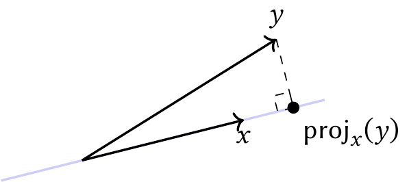
3.4 Projection

In linear models, we will frequently find the projection of vectors onto a space.

Definition 3.15 (Orthogonal projection onto a vector) For any vectors \(x\) and \(y\) in the same space, where \(\|x\|_2 \neq 0\), the orthogonal projection of \(y\) onto \(x\) is the vector \[ \proj_x(y) = \frac{x}{\|x\|_2^2} x\T y. \]

This definition appears arbitrary, but it has very useful properties.

Figure 3.1: Projection of \(y\) onto \(x\), where both vectors are in \(\R^2\). The blue line indicates \(\vspan(x)\), and the dot is the projection.

Theorem 3.2 (Properties of the projection) Given two vectors \(x\) and \(y\),

The residual vector \(r = y - \proj_x(y)\) is orthogonal to all vectors in \(\vspan(x)\), including \(\proj_x(y)\). The projection is hence often called the orthogonal projection.
The projection \(\proj_x(y)\) is the unique vector in the span of \(x\) that is nearest to \(y\). That is, \[ \proj_x(y)= \argmin_{u \in \vspan(x)} \|u - y\|_2. \]

Proof. First, note that the projection is in \(\vspan(x)\) because it is a scalar (\(x\T y / \|x\|_2^2\)) times \(x\) (see Definition 3.3).

Next, consider the residual vector. Let \(u = x / \|x\|_2\), so \(\|u\|_2 = 1\); this will simplify the algebra. Because \(u\) is a simple rescaling of \(x\), \(\vspan(u) = \vspan(x)\), and so \(\proj_x(y) = \proj_u(y)\). Then consider the inner product \((au)\T r\) for any scalar \(a \in \R\): \[\begin{align*} (au)\T r &= (au)\T (y - \proj_u(y))\\ &= (au)\T (au, y - u\T y u)\\ &= (au)\T y - (au)\T (u\T y u)\\ &= a u\T y - a (u\T y) u\T u\\ &= 0, \end{align*}\] because \(u\T u = \|u\|_2 = 1\). Hence \(r\) is perpendicular to any vector \(au \in \vspan(u)\), and equivalently, any vector in \(\vspan(x)\).

Finally, again consider any vector \(au\) for scalar \(a \in \R\). The squared Euclidean distance is \[\begin{align*} \|y - au\|_2^2 &= \|r + \proj_u(y) - au\|_2^2\\ &= \|r\|_2^2 + \|\proj_u(y) - au\|_2^2. \end{align*}\] This holds by the Pythagorean theorem (Exercise 3.2) because the two terms are orthogonal. It follows that the squared distance is bounded below by \(\|r\|_2\), and only attains this value for the unique \(a\) such that \(au = \proj_u(y)\).

One can also prove these properties geometrically, as in Figure 3.1. We can see that any other point in \(\vspan(x)\) (the blue line) would be farther from \(y\) than the marked point, which is the perpendicular projection.

These results let us project vectors onto a one-dimensional space: the space spanned by a single vector. To extend them to higher dimensions, consider a space spanned by multiple basis vectors. To project onto this space, we’ll need to extend Definition 3.15.

Definition 3.16 (Orthogonal projection onto a matrix) Consider a space in \(\R^p\) spanned by vectors \(\{x_1, x_2, \dots, x_n\}\). We can form a \(p \times n\) matrix \(X\) whose columns are the basis vectors. Then the orthogonal projection of a vector \(y \in \R^p\) onto \(X\) is \[ \proj_X(y) = X (X\T X)^{-1} X\T y. \] The matrix \(X (X\T X)^{-1} X\T\) is known as the projection matrix, because multiplying any vector by this matrix projects it into the column space of \(X\).

If the basis vectors are orthogonal and \(X\) is square, then \(X\) is orthogonal (Definition 3.13) and the projection is \[ \proj_X(y) = X X\T y. \]

In the case where \(n = 1\), we can see this reduces to Definition 3.15. The proof of Theorem 3.2 can also be directly extended to show equivalent properties for projection onto a matrix.

Projection matrices have several useful properties.

Theorem 3.3 (Properties of the projection matrix) Consider a projection matrix \(H\), as defined in Definition 3.16.

\(H\) is idempotent: for any vector \(x\), \(Hx = HH x\).
\(H\) is symmetric: \(H = H\T\).

Proof. See Exercise 3.3.

Theorem 3.4 (Orthogonal complement) Consider a projection matrix \(H\) that projects vectors into the column space of \(X\), as defined in Definition 3.16. The matrix \(I - H\) projects vectors into the orthogonal complement of the column space of \(X\): the space of all vectors orthogonal to all vectors in the column space of \(X\).

Proof. Consider two vectors \(x\) and \(y\). We project one into the column space of \(X\) and one into the orthogonal complement, then take their inner product: \[\begin{align*} (H x)\T ((I - H) y) &= (H x)\T (y - H y)\\ &= x\T H\T y - x\T H\T H y\\ &= x\T H y - x\T H H y\\ &= 0. \end{align*}\]

3.5 Eigenvectors and eigenvalues

Definition 3.17 (Eigenvectors and eigenvalues) Consider an \(n \times n\) square matrix \(X\). An \(n\)-vector \(a\) is an eigenvector if \[ Xa = \lambda a, \] where the scalar \(\lambda\) is known as the eigenvalue. The set of all eigenvalues for a matrix is called its spectrum.

If \(a\) is an eigenvector and \(c \neq 0\) is a scalar, then \(ca\) is an eigenvector. Consequently, we usually only deal with the normalized eigenvectors, which are scaled so that \(\|a\|_2 = 1\). It also follows that if \(a\) is an eigenvector, \(-a\) is also an eigenvector; we treat these as the same eigenvector.

TODO discuss number of unique eigenvectors, column rank, etc.

Theorem 3.5 (Eigendecomposition) An \(n \times n\) square matrix \(X\) can be factorized as \[ X = U D U^{-1}, \] where \(U\) is an \(n \times n\) matrix whose columns are the eigenvectors of \(X\), and \(D\) is a diagonal matrix whose diagonal entries are the corresponding eigenvalues of \(X\). This factorization is called the eigendecomposition.

Proof. By Definition 3.17, \(X a = \lambda a\). Consequently, forming all possible eigenvectors and eigenvalues into matrices, \(X U = U D\). Multiply on the right by \(U^{-1}\) to obtain the desired result.

Theorem 3.6 (Orthogonality of eigenvectors) When \(X\) is symmetric, its eigenvectors \(\{u_1, u_2, \dots, u_n\}\) are orthogonal. Consequently, the matrix of eigenvectors \(U\) can be constructed to be orthonormal.

Proof. Consider two eigenvalues \(d_1 \neq d_2\) with eigenvectors \(u_1\) and \(u_2\). By Definition 3.17, we can expand \(d_2 u_1\T u_2\) as \[ d_2 u_1\T u_2 = u_1\T X u_2, \] and we can expand \(d_1 u_1\T u_2\) as \[ d_1 u_1\T u_2 = (X u_1)\T u_2 = u_1\T X u_2, \] because \(X\T = X\) in a symmetric matrix, so the two expressions are the same. Since \(d_1 \neq d_2\), the only way for these two to be equal is if \(u_1\T u_2 = 0\), showing they are orthogonal.

We must also prove the eigenvalues are distinct, i.e. \(d_i \neq d_j\) for all \(i \neq j\). This is more involved; see Gentle (2017), section 3.8.10.1.

Theorem 3.7 (Spectrum of an inverse) If the \(n \times n\) square matrix \(X\) has an eigendecomposition and none of its eigenvalues are zero, then it is invertible and its inverse is \[ X^{-1} = U D^{-1} U^{-1}, \] where \(U\) and \(D\) are defined as in Theorem 3.5. Because \(D\) is diagonal, its inverse is diagonal, where the diagonal entries are the reciprocals of the eigenvalues.

Consequently, the inverse of \(X\) itself can be eigendecomposed, and its eigenvalues are the reciprocal of the eigenvalues of \(X\).

Proof. TODO

Finally, we can use these results to show that for symmetric matrices, the eigenvalue spectrum provides us bounds on how the matrix transforms vectors. This gives us an important tool to describe how a matrix acts upon different vectors and find worst-case scenarios.

Theorem 3.8 (Spectral bounds on transformations) When \(X\) is a symmetric \(n \times n\) matrix with orthonormal eigenvectors and ordered eigenvalues \(d_1 > d_2 > \dots > d_n\), \[\begin{align*} \max_{\|a\|_2 \neq \zerovec} \frac{a\T X a}{\|a\|_2^2} &= d_1\\ \min_{\|a\|_2 \neq \zerovec} \frac{a\T X a}{\|a\|_2^2} &= d_n. \end{align*}\] The values of \(a\) attaining the maximum and minimum are in \(\vspan(u_1)\) and \(\vspan(u_n)\) respectively.

Proof. We can expand this as: \[ \frac{a\T X a}{\|a\|_2^2} = \frac{a\T UDU\T a}{\|a\|_2^2}. \] Let \(y = U\T a\). Then we can write this as \[\begin{align*} \frac{a\T X a}{\|a\|_2^2} &= \frac{y\T D y}{\|a\|_2^2}\\ &= \frac{\sum_{i=1}^n d_i y_i^2}{\|a\|_2^2}. \end{align*}\] As \(\|y\|_2^2 = \|U\T a\|_2^2 = \|a\|_2^2\), for a fixed \(\|a\|_2\), the numerator is maximized by having \(y_1 > 0\) and all other \(y_i = 0\). Then \(y_1^2 = \|a\|_2^2\), so the ratio is \(d_1\). The minimum can be found with the same logic in reverse.

To obtain \(y_1 > 0\) with all other \(y_i = 0\), \(a\) must be orthogonal to \(u_2\) through \(u_n\), and hence parallel to \(u_1\), showing that \(a \in \vspan(u_1)\). Again, the same applies for the minimum.

Theorem 3.9 (Eigenvalues and positive definiteness) A symmetric matrix \(X\) is positive definite if all of its eigenvalues are positive. It is positive semidefinite if all its eigenvalues are nonnegative.

Proof. Apply Theorem 3.8 to the definition of positive definiteness, Definition 3.14.

3.6 Random vectors and matrices

A random vector is a vector whose elements are random variables. By convention, we write random vectors in uppercase and index their elements with subscripts, so \(Y = (Y_1, Y_2, \dots, Y_n)\T\) is a random vector with \(n\) elements.

Expectations are defined elementwise.

Definition 3.18 (Expectation of random vectors) For a random vector \(Y\) with \(n\) elements, \[ \E[Y] = \begin{pmatrix} \E[Y_1]\\ \E[Y_2] \\ \vdots \\ \E[Y_n] \end{pmatrix}. \]

We can apply the conventional definition of variance for scalar random variables, \(\var(X) = \E[(X - \E[X])^2]\), to random vectors.

Definition 3.19 (Variance of random vectors) The variance of a random vector \(Y\) with \(n\) elements is the \(n \times n\) matrix \[ \var(Y) = \E\left[(Y - \E[Y])(Y - \E[Y])\T\right]. \]

Similarly, we can extend the covariance of two random vectors.

Definition 3.20 (Covariance of random vectors) If the random vector \(X\) has \(n\) elements and the random vector \(Y\) has \(m\) elements, then \[ \cov(X, Y) = \E\left[(X - \E[X]) (Y - \E[Y])\T \right] \] is an \(n \times m\) matrix giving the covariance between each pair of elements of the two random vectors.

3.7 Exercises

Exercise 3.1 (Nonnegativity of norms) Using the properties in Definition 3.6, prove that norms are nonnegative: \(p(x) \geq 0\) for all \(x \in \R^n\).

Exercise 3.2 (Pythagorean theorem) Given two vectors \(x\) and \(y\) in \(\R^n\), use Definition 3.7 to show that \[ \|x + y\|_2^2 = \|x\|_2^2 + \|y\|_2^2 \] if and only if \(x\T y = 0\).

Interpret this geometrically. Let the origin, \(x\), and \(y\) form the vertices of a triangle, and indicate what property of the triangle corresponds to \(x\T y = 0\).

Exercise 3.3 Prove Theorem 3.3.

Exercise 3.4 (Properties of random vectors) Let \(X\) and \(Y\) be random vectors. Prove the following properties:

\(\E[aX + b] = a \E[X] + b\), where \(a\) is a fixed scalar and \(b\) is a fixed vector.
\(\var(a\T X) = a\T \var(X) a\), where \(a\) is a fixed vector of appropriate dimension.

You may use any results about the properties of expectations and variances of scalar random variables.

Exercise 3.5 (Manipulating a multivariate normal) Let \(X\) be a multivariate normal random variable: \(X \sim \normal(\mu, \Sigma)\), where \[\begin{align*} \mu &= \begin{pmatrix} 0 \\ 2 \\ 1 \end{pmatrix} & \Sigma &= \begin{pmatrix} 1 & 0 & 0.5 \\ 0 & 1 & 0 \\ 0.5 & 0 & 1 \end{pmatrix} \end{align*}\]

Define the quantity \[ W = \frac{2 X_1 - 2 X_2 - X_3}{\sqrt{5}}. \] What is its distribution? Use appropriate matrix operations to find its mean and variance.
Define the fixed (not random) matrix \[ A = \begin{pmatrix} 1 & 0 & 1 \\ 1 & 0 & 1 \end{pmatrix}. \] What is the distribution of \(Y = A X\)? Are the components of \(Y\) independent of each other?

Exercise 3.6 (Positive semidefiniteness of variance) Let \(X\) be a \(p\)-dimensional random vector. Show that covariance matrix \(\var(X)\) is positive semidefinite (Definition 3.14).